The Data Source Specification Panel

Content

Supported data formats and data sources
The 'Input Data' panel
The 'active fields' pop-up dialog
The 'advanced options' pop-up dialog
User specified binnings and discretizations
Value groupings and variant elimination
Name mappings
Taxonomies (hierarchies)
Joining with auxiliary tables
Computed data fields
Transactional and streaming data

Supported data formats and data sources

Synop Analyzer is able to read data from the following data sources:

• Tables or views from all database management systems (DBMS) which support the JDBC data exchange interface.
• Microsoft Access^© tables stored as MDB files .
• Spreadsheets in the Microsoft Excel^© formats .xlsx and .xls. For importing data from spreadsheets with a complex structure of data, meta data, formula and textual explanation cells, see Importing data from spreadsheets .
• Flat text files in which the first row optionally contains the column names and the following rows the column values. The columns must be separated by a separator character such as <TAB>, '|', ',', ';', or ' ' .
• XML files. Here, the first repeatedly occurring XML tag in the hierarchy level directly below the document's root element is interpreted as the data container which contains the information of one data record. The field names of the data record are automatically detected from the attributes and the sub-tags of that data record tag. .
• Data retrieved via a web API such as the Google Analytics API.
• Files in the Synop Analyzer-proprietary compressed .iad data format .

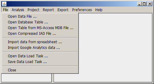
A new data source can be opened by clicking on the item File in Synop Analyzer's main menu:

Once you have opened a data source and you have specified some additional data import settings such as data field usage types, joins with auxiliary data, field discretizations, or computed fields, you can save these settings by clicking on File → Save data load task in Synop Analyzer's main menu. This will create a parameter file in XML format. You can later re-open this XML file via File → Open data load task.

The 'Input Data' panel

When a data source has been selected using the menu item File, an input data specification panel opens up in the left part of the Synop Analyzer screen. By pressing the Start button in the middle of that panel, the data are read into your computer's memory. Once this process is finished, the buttons in the lower part of the panel become enabled. Using these buttons, you can start Synop Analyzer's different data analysis and exploration modules.

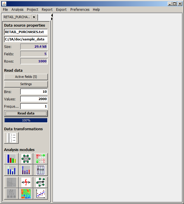
When reading a data source, Synop Analyzer uses certain predefined settings and makes some assumptions as to the desired usage of the single data fields. The settings can be introspected and modified using the menu item Preferences → Data Import Preferences. Further assumptions and parameter settings are directly shown in the input data panel. Some basic parameters are visible in the upper part of the panel:

• Active fields:
  This button opens a dialog window in which active and inactive data fields can be selected and the roles of the active fields in the subsequent analysis steps can be specified. A more detailed description is given in The 'active fields' pop-up dialog.
• Settings:
  This button opens a dialog window in which active and inactive data fields can be selected and the roles of the active fields in the subsequent analysis steps can be specified. A more detailed description is given in The 'settings' pop-up dialog.
• Bins:
  Several data exploration modules of Synop Analyzer display histogram charts of the data field's value distributions. For that purpose, the values of numeric data fields must often be discretized into a manageably small number of value ranges (intervals), otherwise the resulting histogram charts would become completely overcrowded. The number given in this parameter input field is the desired default number of histogram bars for all numeric data fields. The choice of the actual interval boundaries as well as the scaling - equidistant or logarithmic - is thereby left to a software heuristics. For single data fields, this behaviour can be overwritten, see User specified binnings and discretizations .
• Values:
  Several data exploration modules of Synop Analyzer display histogram charts of the data field's value distributions. For that purpose, the less frequent values of textual data fields must sometimes composed into groups, otherwise the resulting histogram charts would become completely overcrowded. The number given in this parameter input field is the desired maximum number of histogram bars for all non-numeric data fields. If the field contains more different values, the most frequent values get their own histogram bin, the remaining values are combined int one single value group called 'others'. For single data fields, this behaviour can be overwritten, see User specified binnings and discretizations .
• Frequency:
  This parameter defines a lower boundary for the number of data records or data groups on which a value of a non-numeric data field must occur for being tracked as a separate field value and a separate bar in histogram charts. Less frequent values will be grouped into the category 'others'.

Hint: You can duplicate a data import panel by right-clicking on the tab header of the panel. This creates a new input data panel in addition to the existing one. The new panel inherits all settings and specifications for importing the data that were specified on the original panel. You can now modify some of these settings in order to generate a second, slightly modified view on the data.

The 'active fields' pop-up dialog

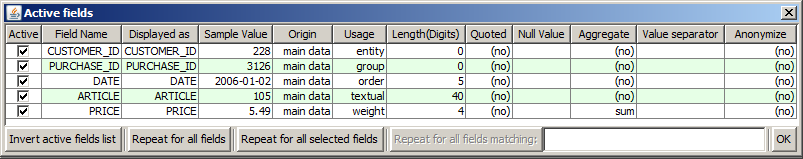
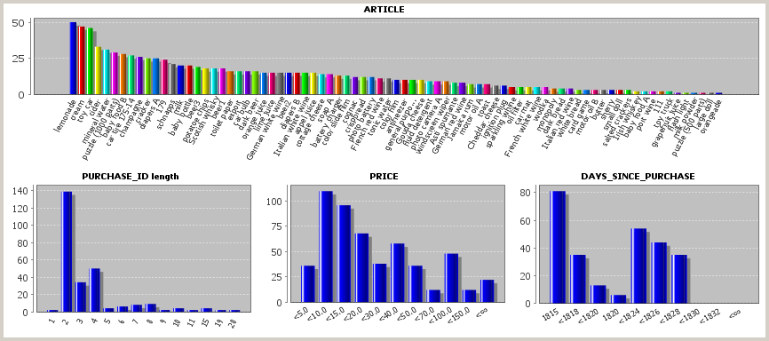
Clicking on the button Select active fields in the input data panel opens a pop-up dialog in which all data fields of the current data source are displayed. The picture below shows the pop-up dialog for the sample data source doc/sample_data/RETAIL_PURCHASES.txt.

In the dialog, you can define several properties for each data field:

• Active:
  Deactivating this check box hides the data field when the data are read. The data source is treated as if the field was not present in the data .
• Field name:
  This table column is non-editable. It displays the original field name as it appear in the data source .
• Displayed as:
  In this table column you can define a new name which will be displayed instead of the original field name in all subsequent analysis results .
• Sample value:
  In this table column, the first value of the data field is displayed .
• Origin:
  This table column is non-editable. It displays the source of the data field. For data fields from the main data source, main data is displayed, joined data for data fields from auxiliary tables which were joined in, computed for computed fields and replaced for data fields which were present in the main data or an auxiliary data source but which were replaced by computed fields .
• Usage:
  In this table column you specify the data type and the usage mode of the corresponding data field. The default is automatic, which means that the field's data type is automatically set to textual, Boolean, numeric or discrete (numeric) based on an analysis of the field's first values, or, if the data source is a relational database, based on the field's data type in the database.
  This default handling can be modified by mouse-clicking into the table cell. On the one hand, one can manually specify the field's data type to be textual, Boolean, numeric or discrete (numeric). Most practical relevance has the case that a data field with purely numeric values is to be treated as textual or group field, for example if the field is an ID or key field, for which the standard numeric field treatment, which involves calculating value ranges and statistics such as mean and standard deviations, would make no sense. In the screenshot above, the ID field ARTICLE has been treated in this way.
  On the other hand, you can specify four specific field usage modes which do not only define the field's data type but also its role and function within the data source. None of these four field usage modes may be set for more than one data field:
  Order denotes a data field whose values are time stamps, dates or another numeric ordering criterion which specifies the time and order at which the other field values of the data record have been recorded. In the screenshot above, the field DATE has been specified as order field.
  Weight specifies a numeric data field whose values contain the price, cost, weight, importance or another quantitative rating number which can be attributed to the corresponding data record. In the screenshot above, the field PRICE has been treated in this way.
  Group should be used for a field which does not contain any independently usable information but serves for marking several adjacent data records as parts of one single data group. In the screenshot above, the field PURCHASE_ID has been marked as group field: it marks several consecutive data sets as parts of one single purchasing transaction. If a group field has been defined, all subsequently generated statistics and analysis results do not count and display data record numbers but data group numbers.
  Entity denotes a second, higher-level grouping of data records on top of the group field. The specification of an entity field is particularly important for sequential patterns analyses . In this case, the group field defines groups of simultaneous events, the entity field defines 'entities' or 'subjects' to which time-ordered series of groups of simultaneous events can be attributed. Typical entity field - group field pairs are customerID and purchaseID, productID and productionStepID, or patientID and treatmentID .
• Length (Digits):
  For non-numeric fields, this is the maximum number of characters within a field's values; longer values will be truncated when reading the data into memory. For numeric fields, this is the numeric precision. For example, if this value is 4, then the number 1.2345 will be read-in as 1.235 because all digits after the fourth one will be rounded away .
• Quoted:
  In this table column the user can tell Synop Analyzer that some or all values of a data field are enclosed into single or double quotes in the data source and that these quotes should be ignored and stripped away when reading the field's values. Note: if all values of a field are enclosed in the same type of quotes, Synop Analyzer automatically recognizes and removes these quotes when reading the data .
• Null value:
  Per default, Synop Analyzer interprets the empty string and the value SQL NULL (when reading from relational databases) as 'no value available'. In real-world data, there are often additional special field values which indicate the absence of a valid value, for example the entry '-' in a name or address field, or the value '1900-01-01' in a data field, or '-1' in a field which should contain positive numbers. Those specific 'placeholder' values should be entered into the table column 'Null value' so that Synop Analyzer can correctly represent the intended purpose of these values .
• Aggregate:
  Once you have defined a group field, n consecutive data sets with identical group field values are treated as one single data group. For each nummeric data field, such a group contains up to n different numeric values. The question now is: how should these single values be aggregated in order to form one single value which can be attributed to the data group? Per default, the sum of all values will be calculated. If you want to define another aggregation method, for example the mean, minimum, maximum, spread (maximum minus minimum), relative spread (maximum minus minimum dividey by mean), count (the number of valid values), or existence (1 if a valid value exists, 0 otherwise), click on the table cell Aggregate and selecte the desired aggregation mode. In the screenshot above, the aggregation function of the weight field PRICE has been set to sum, and consequently, the field has been renamed to 'PurchaseValue' as the field now represents the total value of each purchase .
  There are more complex aggregation methods which involve the values of other data fields as aggregation criteria. The method Value at which XXX is maximum, for example, selects the field value of that data record within the data group at which the data field XXX assumes its maximum value within the data group.
• Value separator:
  In this column you should enter a value if the corresponding data field contains set-valued entries, for example entries of the kind cream;diapers;mineral water;baby food. In these cases, the software must be told that the entry should not be treated as one single information but as a set of several single bits of information, that means in our example the set of the four values cream, diapers, mineral water and baby food. In order to achieve this, enter the separator character into the Value separator column, in our example the character ;. Once a separator character has been defined, eventually present braces around the entire expression are automatically identified as set indicators and ignored when extracting the single values of the set. .
• Anonymize:
  Sometimes analysis results created on confidential data are to be distributed to a larger receiver group which is not authorized to see all parts of the data. For this case, Synop Analyzer offers the possibility to anonymize certain field names and/or these fields' values before reading the data and creating analysis results. For each data field, the anonymization level can be set individually. There are three modes: one can anonymize the field name, the field's values or both. If you permanently store the imported data as a compressed .iad file, this file only contains the anonymized data and not the original values. Hence, you can distribute the .iad file together with the analysis results .

Duplicating data fields

Sometimes it is desirable to use one single data field from the original data in two different ways in Synop Analyzer. For example, you could use the time stamp of a transaction within a transactions data collection both as grouping criterion (usage 'group') and as time order field (usage 'order'); or you could use and display one single date field with the two different aggregation modes 'minimum' and 'maximum' in order to show the date of the first and the last transaction of a customer.

In Synop Analyzer, you can duplicate a data field by right mouse click on the table row representing the data field in the pop-up dialog Select active fields. In a second pop-up dialog you will then be asked to specify the name of the new copy of the original data field. Make sure that the new display name is unique:

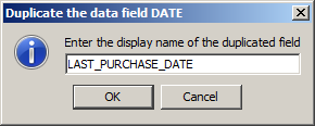
After closing the field name dialog the duplicated data field will appear as a new row in the table of all available data fields. You can then specify the desired usage type, aggregation mode and other desired properties of the duplicated field.

The screenshot below shows a practical example in which defining duplicated fields is very helpful: on the sample data sample_data/RETAIL_PURCHASES.txt we have defined the field CLIENT_ID as the grouping criterion. The field DATE has been duplicated, renamed into FIRST_PURCHASE_DATE and LAST_PURRCHASE_DATE and furnished with the aggregation modes 'minimum' resp. 'maximum'. Similarly, the field ARTICLE has been duplicated, renamed into CHEAPEST_ARTICLE and MOST_EXPENSIVE_ARTICLE and furnished with the aggregation modes 'value at which PRICE is minimum' resp. 'value at which PRICE us maximum'. wurden dupliziert, umbenannt in ERSTES_KAUFDATUM und LETZTES_KAUFDATUM und mit der jeweils passenden Aggregierungsfunktion (Minimum bzw. Maximum) versehen. Schließlich wurde noch das Datenfeld ARTIKEL dupliziert, umbenannt in BILLIGSTER_ARTIKEL und TEUERSTER_ARTIKEL und mit der Aggregierung 'Wert, bei dem PREIS minimal ist' bzw. 'Wert, bei dem PREISmaximal ist' versehen.

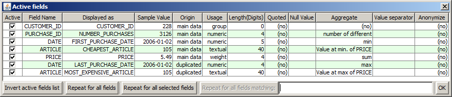
When you import and display the data in Synop Analyzer in this way, the displayed data contain one single row per customer. The data row contains the ID of the customer, his or her total number of purchases, the total amount of money spent so far, the cheapest and the most expensive article purchased so far, and the date of the first and the last purchase.

Hints for minimizing memory requirements and for maximizing processing speed

• Textual data fields with many (more than ca. 5000) different values have high memory requirements and reduce the speed of following analysis steps. Therefore, free text fields and ID or key fields should be deactivated in the 'select active fields' dialog whenever possible .
• Sometimes you still want to keep a key field with tens of thousands or even millions of different values, for example because your analysis aims at creating small subsets of the original data and in these data subsets you need the key attribute for unambiguously identifying each selected data record. The selection of a target group of customers for a marketing campaign is such an example: here, you want to keep the 'customerID' field even if it contains millions of different IDs. In this case you should mark the data field as group field and not as textual field: internally, the treatment and memory storage model of group fields is optimized for many different values, the treatment of textual fields is not .
• For numeric data fields with many different values, the memory requirements for storing them heavily depends on the numeric precision with which the field values are read-in. Such a data field, when read-in with a numeric precision of 7, can consume up to 1000 times more memory than the same data field read-in with a precision of 4. A precision of more than 3 to 5 digits is rarely needed for analysis and data mining tasks. Therefore, on large data you should reduce the numeric precision to the minimum acceptable number .

The 'Settings' pop-up dialog

Many more advanced options for customizing the data preparation and data importing process are accessible via the pop-up panel Settings. The panel is organized into seven 'tabs' or pages, which will be described one by one in the following sections of this document.

The 'Reading Options' tab

In the upper part of the first tab named Reading options, one can specify whether the binary data object which has been composed in the computer's main memory is also stored permanently in the form of an .iad file. The iad data format is an Synop Analyzer-proprietary data format; it contains a compressed binary representation of the input data as well as all data preprocessing and data joining steps defined in the input data panel. An iadcan be loaded from disk very quickly - much faster than the time it took to read the data from the original data sources.

If only the data preparation and data import settings but not the imported data themselves are to be stores, one can activate the check box Store the load task as XML file. This option has the advantage that one can repeatedly re-load the must current data snapshot from the original data source without to be obliged to re-enter the data preparation and data import settings.

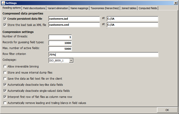
In the lower part of the tab you can modify various predefined settings for the process of reading the data into the computer's memory:

• Number of threads:
  Specify an upper limit for the number of parallel threads used for reading and compressing the data. If no number or a number smaller than 1 is given here, the maximum available number of CPU cores will be used in parallel.
• Records for guessing field types:
  When reading input data from flat files or spreadsheets, the data source does not provide meta data information on the types of data (integer, Boolean, floating point, textual) to be expected in the available data columns. Therefore, a presumable data type has to be derived from looking at the data fields actual content. The parameter 'number of records for guessing field types' determines, how many leading data rows are read from the data source for guessing data field types.
• Max. number of active fields:
  If a data source contains a large number of data fields, it is helpful for the clarity and speed of any subsequent analysis steps to concentrate on not more than 40 to 50 of the data fields. By entering a number smaller than the current number of active data fields, you ask the software to find a subset of all data fields which contains as much as possible of the information contained in the entire data. This will be reached by deactivating fields with many missing values, almost unique-valued fields or almost single-valued fields, and by dropping all but one field from each tupel of highly correlated fields such as AGE and DATE_OF_BIRTH .
• Row filter criterion:
  Here, you can define a data row filter criterion. This can be specified in the form of a percentage; for example, the filter 5% means that a random sample of about 5% of the entire data will be drawn. The filter !5% creates the inverse sample which contains exactly those data records which are not part of the 5% sample. If your data source is a database table, you can also submit the filter criterion in the form of a SQL WHERE clause; for example, WHERE AGE<40 means that only those data sets are to be read in which the field AGE has a value of less than 40.
• Codepage:
  The codepage (encoding scheme) in which the input data are encoded defines the way in which bits and bytes in the source data are interpreted as letters and symbols. Synop Analyzer's standard codepage is the US and Western European default ISO_8859_1, which is a 1-byte codepage (1 byte per character). Another frequently used code page is UTF-16 (2 or more bytes per character).
• Allow irreversible binning:
  If this check box is marked, numeric data fields can be discretized into a small number of intervals, and the original field values are irreversibly replaced by interval indices. For example, the value AGE=37 might be replaced by AGE=[30..40[, and in the compressed data, the precise value 37 will be irreversibly lost. This discretization can significantly reduce the memory requirements of the data.
• Store and reuse internal dump files:
  When reading data from flat files or database tables, a temporary buffer object is created for each data field. Storing and reusing these temporary objects can considerably speed up the data reading process in subsequent data reading steps from the same data source.
• Save the data as flat text on the client:
  When reading data from a remote text file or database table, copy the data in the form of a flat text file into the current working directory on the local machine. This can speed up subsequent data reading steps if the bandwidth to the remote data server is limited.
• Automatically suppress key-like fields:
  Key-like fields are non-numeric data fields in which (almost) every data record has a unique value. This option automatically sets the usage mode of all those data fields which have not been specified as group field to 'inactive'.
• Automatically suppress single-valued fields:
  Single-valued fields are data fields in which (almost) every data record has the same value. If this checkbox has been marked, the usage mode of all those data fields is automatically set to 'inactive'.
• Interpret first row of flat files as column name row:
  Per default, the first row of a flat text file will be interpreted as head row containing the column names. You should deactivate this option when reading flat files which do not have a head row.
• Automatically remove leading and trailing blancs in field values:
  f this option is activated, leading and trailing spaces are automatically removed when importing the data.

User specified binnings and discretizations

This tab provides the means for a field-specific modification of the default settings of

• how many different field values of non-numeric fields are treated as separate values and which values are grouped into 'others'
• how many value ranges (intervals) are used to display the value distributions of numeric fields in histogram charts and what are the interval boundaries.

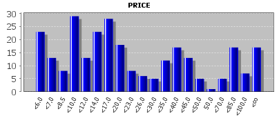
In the following, we want to demonstrate this using the sample data RETAIL_PURCHASES.txt. If these data are imported into Synop Analyzer as described in the 'active fields' pop-up dialog, with PRICE as weight field and PURCHASE_ID as group field, then the values of the field PRICE will be partitioned into the following ranges:

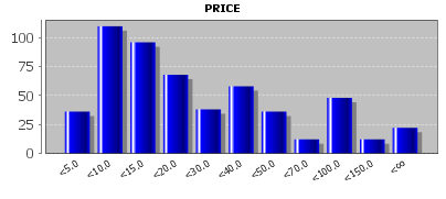
This range partition shall now be replaced by the 11 ranges with the boundaries 5, 10, 15, 20, 30, 40, 50, 70, 100 and 150. We open the tab Field discretizations and enter the following string into the field Interval bounds (numeric fields only): 5 10 15 20 30 40 50 70 100 150. Then we finish the specification by pressing <TAB> or <Enter> and press Add. The tab now looks like this:

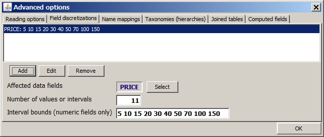
Each series of interval boundaries such as 5 10 15 20 30 40 50 70 100 150 which has been specified for a field discretization is stored in a 'interval boundaries history' store in the preference settings of Synop Analyzer. You can access the the 50 most recently used interval boundary sets from the pull-down selection box at the right side of the input field for interval boundaries.

If we close the pop-up dialog now using OK and re-open an analysis view which shows value distribution histograms, the histogram for the field PRICE shows the desired value ranges:

You can delete manually defined value range definitions by means of Delete and modify them using Edit.

Value groupings and variant elimination

This tab provides the means for reducing the set of field values of a textual data field. The most important application areas are:

• If the data contain misspelled entries or different names for identical things, for example the variants TOYOTA COROLLA, Corolla, Corrola, Toyota Corolla GT 2.0, T.Cor. für das car mark Toyota Corolla.
• If the information contained in the data field are too fine-grained and ought to be summarized into a smaller number of groups or categories, for example the professions supermarket articles apples Granny Smith, apples Golden Delicious, apples Braeburn and apples Idared to the group apples.

In Synop Analyzer, you can define several value groupings or variant eliminations within the tab Variant elimination, and each of them can be activated for one or more data fields. Per default, all variant eliminations defined when importing a certain input data source are stored as a part of the 'data load task', that means the XML file which stores all settings and user-defined specifications which have been performed for the input data source. But using the button Save selected as file you can also save a variant elimination as a data-independent persistent XML file. This file can later be loaded and activated for a new data source using the button Load from file. This mechanism enables the creation of a data-independent 'knowledge base' of spelling variants for specific application areas, for example a data-independent knowledge base of Toyota car names.

Each variant elimination consists of the following parts:

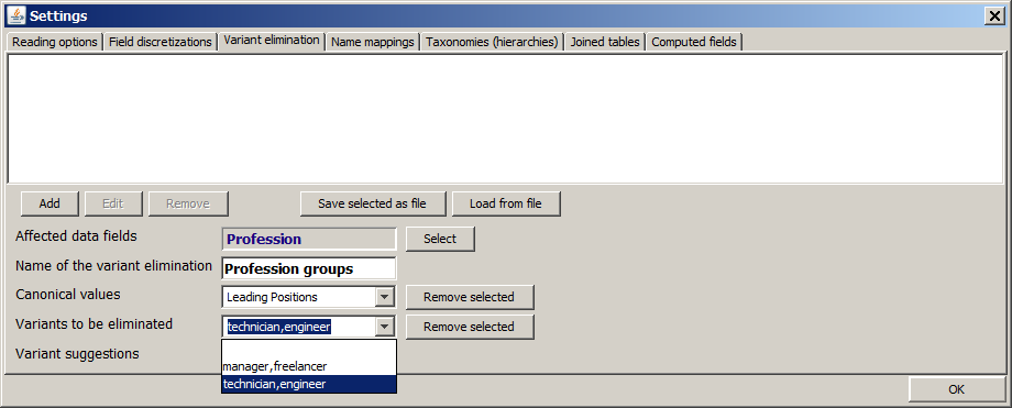
• The data fields on which the variant elimination is to be applied. In the example shown above, which is built on the sample data doc/sample_data/customers.txt, the variant elimination shall be applied to one single field, Profession.
• A unique name for the variant elimination. In the example shown above, we use the name Profession groups.
• The specification of at least one 'canonical form' or group value. In the example shown above, we have defined one single group value called Leading Positions.
• The definition of several variants or at least one variant pattern for each value group. In the example shown above, we wanted to combine the two values manager,freelancer and technician,engineer into the new group value Leading Positions. The variant specifications could also contain regular expressions; for example, the character * stands for 0, 1 or more arbitrary characters; the expression [Aa] stands for 'either A or a', the expression [a-z] for exactly one lower case letter. In order to make it easier to work with this feature for users which are not familiar with regular expressions, Synop Analyzer interprets each appearance of '*' as a general wildcard representing zero or more arbitrary characters. That means, the expression Tech* is interpreted as 'All strings starting with Tech'; in correct regular expression syntax we would have to write that as as Tech.*, which is also possible in Synop Analyzer.
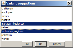
  The variants can either be typed in one by one using the input field Variants to be eliminated, or one can select the desired values from an lexically sorted list of all different field values of the affected data field which is opened by pressing the button Variant suggestions. However, this latter way is only available if the input data have been read in by Synop Analyzer before using the button Read data in the left column of the main screen. In our example shown above, the button Variant suggestions would show us, if we have read in the data customers.txt before, the following list, from which we can select the desired values by pressing the OK button:
  
• Finally we have to specify whether the original data field values are to be replaced by the value group names matching them, or whether they are to remain in the data in addition to the newly added value group names. This is done by means of the check box Keep also the original field values.

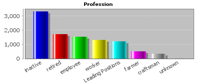
Once defined, the variant elimination settings will be applied to all subsequent data reading processes on the current input data. In our example, the two values manager,freelancer and technician,engineer of the data field Profession are replaced by the group value Leading Positions:

Name mappings

This tab provides the means for assigning more cleary understandable alias names to the values of a textual data field. These names can be read from an auxiliary file or database table which must contain at least two columns: one column must contain values which exactly correspond to the existing values of the textual field, the second column must contain the desired alias names for these values.

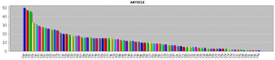
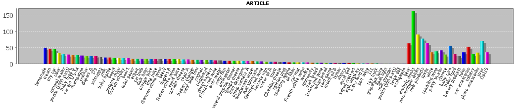
In the following, we want to demonstrate this using the sample data RETAIL_PURCHASES.txt. If these data are imported into Synop Analyzer as described in the 'active fields' pop-up dialog then the field ARTICLE contains hardly understandable 3-digit ID numbers. We would like to replace these numbers by textual article names.

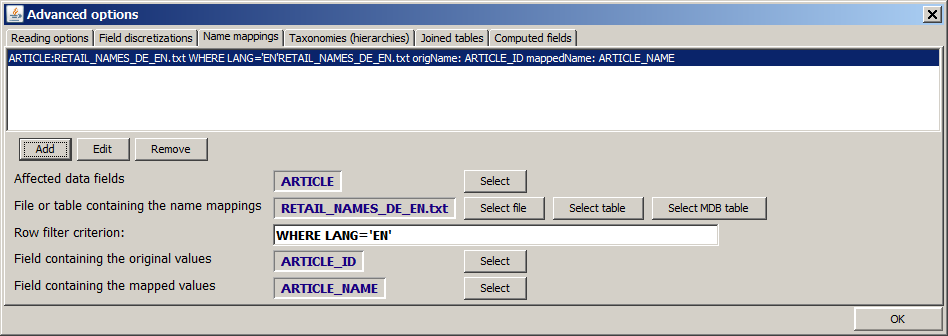
A list of English and German article names is available in form of the file doc/sample_data/RETAIL_NAMES_DE_EN.txt. This file contains three columns: ARTICLE_ID, ARTICLE_NAME and LANG. ARTICLE_ID contains the same article identifier number which occur in the main data and LANG contains the two language identifiers DE and EN. We open the tab Name mappings within the Advanced options pop-up window and insert the entries shown in the picture below in the lower gray part of the tab. Then we press the Add button. The tab should look like this now:

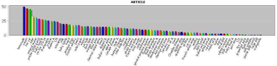
If we close the pop-up dialog now using OK and re-open an analysis view which shows value distribution histograms, the histogram for the field ARTICLE shows the desired textual values:

You can delete manually defined name mapping definitions by means of Delete and modify them using Edit.

Taxonomies (hierarchies)

This tab provides the means for adding hierarchical grouping information to the values of a textual data field. Hierarchies, also called 'taxonomies', can be read from an auxiliary file or database table which must contain at least two columns: one column must contain the lower-level ('child') part of a hierarchy relation, the other column the higher-level ('parent') part.

In the following, we want to demonstrate this using the sample data RETAIL_PURCHASES.txt. We assume that these data have been imported into Synop Analyzer and enriched with name mapping information as described in section Name mappings. We would like to add article group and article department information to the article names.

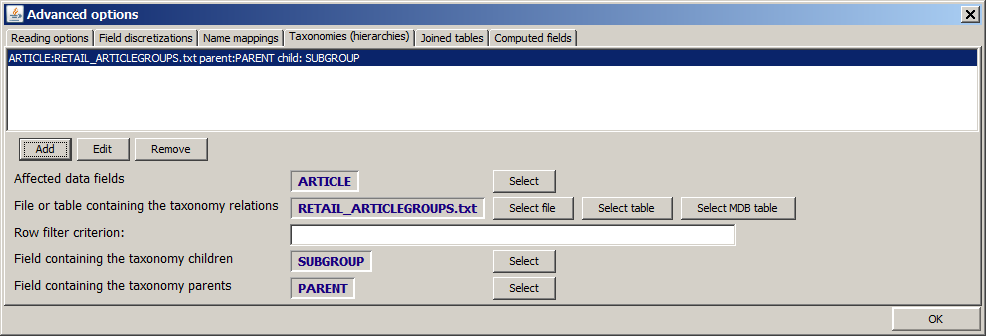
A list of article group and department information is available in form of the file doc/sample_data/RETAIL_ARTICLEGROUPS_DE_EN.txt. This file contains the columns: PARENT and SUBGROUP, which are easily identified as parent and child column. We open the tab Taxonomies within the Advanced options pop-up window and insert the entries shown in the picture below in the lower gray part of the tab. Then we press the Add button. The tab should look like this now:

If we close the pop-up dialog now using OK and re-open an analysis view which shows value distribution histograms, the histogram for the field ARTICLE shows new article group values and department values in addition to the existing article names. (Per default, the Synop Analyzer histograms show only up to 80 histogram bars. You can increase this value to 100 in the pop-up dialogs Preferences → Univariate Preferences and Preferences → Multivariate Preferences in order to obtain the result shown below.)

You can delete manually defined taxonomy definitions by means of Delete and modify them using Edit.

Joining with auxiliary tables

This tab provides the means for appending new data fields (columns) to an existing data source which has been opened in Synop Analyzer. The values in the new fields are obtained from a second data source; they are merged into the main data source via a foreign key - primary key relation between a field in the main data source and a field in the second data source. That means, the main data source must contain a data field ('foreign key field') whose values are the values of a primary key field in the second data source. It is not neccessary that the primary key field has been explicitly specified as primary key field within the second data source, it is sufficient that the field is a 'de-facto' key field in the sense that no value of the field occurs identically in more than one data row.

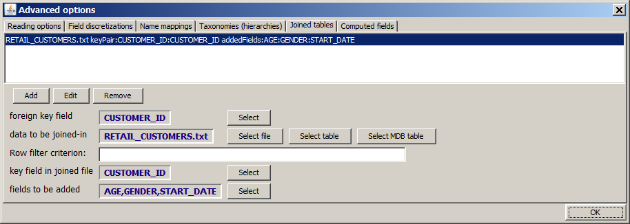
In the following, we want to demonstrate this using the sample data RETAIL_PURCHASES.txt. We assume that these data have been imported into Synop Analyzer and enriched with name mapping information as described in section Name mappings. We would like to add customer master data to these data. A master data file is available in doc/sample_data/RETAUL_CUSTOMERS.txt. It contains the data fields AGE, GENDER and START_DATE (the latter being the date at which the customer loyalty card was handed out). The connection to the main data source is established via the foreign key - primary key pair CUSTOMER_ID (foreign key field in RETAIL_PURCHASES.txt) and CUSTOMER_ID (primary key field in RETAIL_CUSTOMERS.txt).

We open the tab Joined tables within the Advanced options pop-up window and insert the entries shown in the picture below in the lower gray part of the tab. Then we press the Add button. The tab should look like this now:

Note: the input field Row filter criterion can be used to make a field which is not a primary key field in the auxiliary data source behave like a primary key field. Imagine that we want to add a customer address field to the main data, but in the address master data there are customers for which we have two or more addresses, labeled by an address counter field ADDRES_NBR which contains a running number 1, 2, 3, etc.. In this form, we cannot join-in address information because for some customers we don't know which address to take. However, if we enter WHERE ADDRESS_NBR=1 into the field Row filter criterion, the address becomes unique and the joining-in canbe performed.

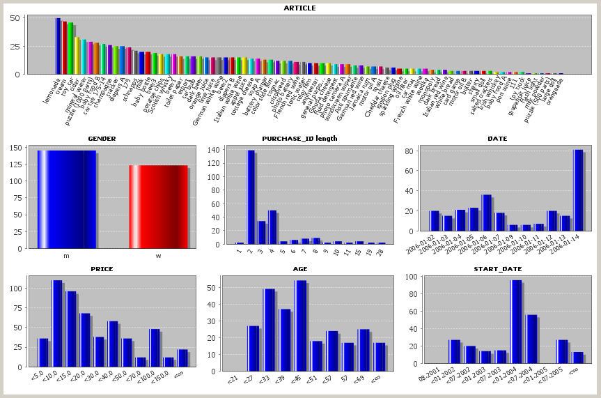
If we close the pop-up dialog now using OK, re-read the data and open an analysis view which shows value distribution histograms, three new histograms for the fields AGE, GENDER and START_DATE appear. These new fields can now be used just as if they had been present in the main data source right from the beginning. And if you persistently save the data as an .iad, the saved data also contains the three new fields.

You can delete manually defined joined data definitions by means of Delete and modify them using Edit.

Computed data fields

This tab provides the means for appending new fields (columns) to an existing data source whose values are the result of applying a computation formula to the values of one or more existing data fields.

In the following, we want to demonstrate this using the sample data RETAIL_PURCHASES.txt. We assume that these data have been imported into Synop Analyzer and enriched with name mapping information as described in section Name mappings. We would like to add a new data field which contains the number of elapsed days between the date of the purchase and the current day at which the data analysis takes place. This information can be calculated from the value of the data field DATE and the current date.

We open the tab Computed fields within the Advanced options pop-up window and insert the entries shown in the picture below in the lower gray part of the tab. Then we press the Add button. The tab should look like this now:

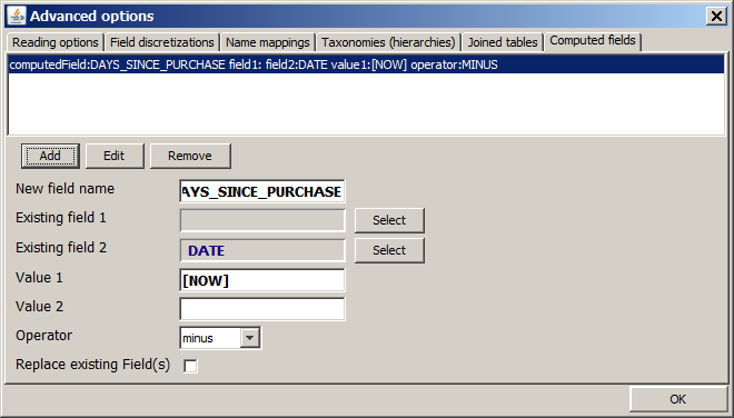
Note: In order to tell the software that the first part of the formula does not depend on the value of a data field, we have clicked in the button Select next to Existing field 1, then we have selected the last, empty entry in the pop-up menu. Without this step, the Add remains grayed-out and unusable.

Note: By activating the check box Replace existing fields you can tell the software that the existing fields involved in the formula should be removed from the data after the computation. However, this is not possible if one of the fields to be removed has been assigned one of the four special roles 'group', 'entity', 'weight' or 'order'. Therefore, the field DATE can not be replaced. One would get an error message if one tried to do so.

Note: The special constant [NOW] is a placeholder for inserting the current date and time of the time the data are read into memory.

If we close the pop-up dialog now using OK, read the data and open an analysis view which shows value distribution histograms, we see the new data field DAYS_SINCE_PURCHASE. In the screenshot below, we have deactivated the existing field DATE using the Visible fields button. Furthermore, we have increased the default number of histogram bars for numeric fields from 10 to 12 (using input field #bins (numeric fields)) before reading the data.

You can delete manually defined computed field definitions by means of Delete and modify them using Edit.

Transactional and streaming data

Automatically recorded mass data from logging systems - for example supermarket cash desk data, web stream data or server log data - often have only two columns: a counter or time stamp column and another column which contains all the information recorded at a certain counter state or time. The sample data file doc/sample_data/CAR_REPAIR.txt is an example for such a type of data. The file contains car read-out data which were recorded when a cars were connected to a testing device at a car repair shop.

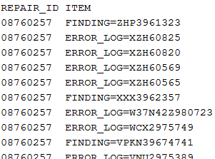
As can be seen from the data extract shown above, the second column contains the read-out information in the form attribute name = attribute value. The first column is the ID column. Its values indicate which data rows belong to one single car read-out.

When the data CAR_REPAIR.txt are read into Synop Analyzer, the field REPAIR_ID should be specified as group field. See section The 'active fields' pop-up dialog for more details.

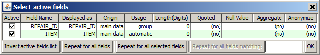
Whenever Synop Analyzer is reading data which contain - apart from a possibly specified group, entity, order and/or weight field - only one single, textual data field, the software checks whether it is able to detect internal structures and groups of information within the single textual field. In particular, Synop Analyzer searches for prefixes of the kind attribute name=, with the aim of identifying several different such prefixes and using them for information grouping.

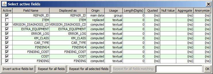
Once the data have been read-in by pressing the button Start in the input data panel, one can introspect the different 'information groups' or prefixes by clicking on the Select active fields button: each prefix group is shown as a separate data field. In the example of the CAR_REPAIR.txt data, 9 such artificial data attributes are detected. The original data field ITEM has been marked as 'replaced':

In following data analysis steps, one can work with the artificial data fields as if they were full blown data fields from the data source. As an example, we show a univariate statistics view in which the value distributions of the artificial data fields can be studied:

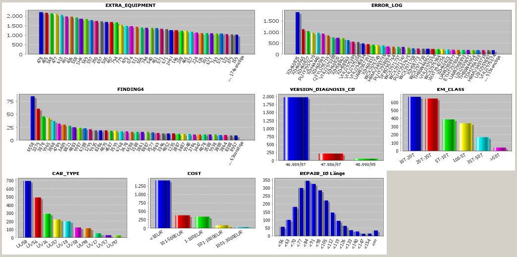
At the end of this section we want to discuss the possible question what the advantage of the two-column 'transactional' data format is. The answer is that this 'slim' data format offers a very flexible possibility to store both set-valued and scalar-valued data attributes in one single flat data structure without any redundancy. In our example, some of the attributes typically contain many different values per repair ID, for example ERROR_LOG, EXTRA_EQUIPMENT or FINDING. Other attributes such as CAR_TYPE or KM_CLASS contain only one value per repair ID. The first group is set-valued (with respect to one repair ID), the second group is scalar-valued. Both groups can be stored together without to introduce redundancies, for example by repeating identical values of scalar-valued attributes.