Data Transformations

Content

Purpose
Aggregating (grouping) data records
Splitting a data source in two parts

Purpose

The 'Data Transformation' functions in the data source panel can be used to transform an existing in-memory data source within Synop Analyzer into one or two new data sources with slightly different properties. The new data sources will be available in Synop Analyzer in addition to the original data source.

At the moment, the following data transformation functions are available:

• : Group data rows: the data records of the original data source are grouped (aggregated) into larger groups. A numeric data field serves as the grouping criterion: a new group begins whenever the value of this data field differs from the previous record's value or the value on the first record of the group by more than a user-defined threshold.
• : Split the data: the original data source is split into two parts. Each data record of the original data is assigned to exactly one of the two new parts. The assignment is performed by means of a random number generator. The data can be split symmetrically (50:50) or asymmetrically.

Aggregating (grouping) data records

This transformation function creates a new data source in which the data records are aggregated into larger groups, each group defining one data record of the new data. Optionally, some of the data fields of the original data source can be suppressed during that transformation.

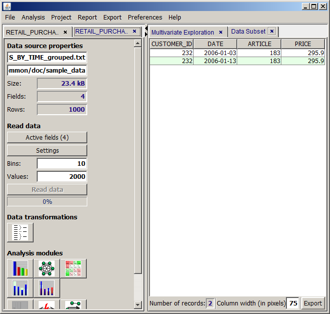
In the following paragraphs, we will demonstrate that function using a concrete example. To that purpose, we open the data doc/sample_data/RETAIL_PURCHASES_BY_TIME.txt and read them into Synop Analyzer using the default settings. The file contains supermarket checkout data: 1000 purchased articles, sorted by the date and time of purchase.

We want to create a list of the most expensive purchase article (and the customer who purchased it) of each week. By clicking the button , we open a pop-up window in which we can specify the parameters for a data aggregation:

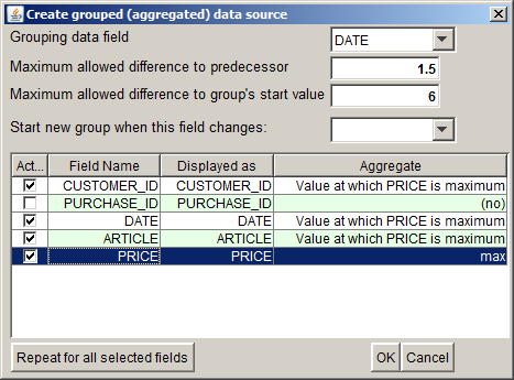
In the screenshot shown abive, we have already performed the following modifications in the panel:

• In ths selection field Grouping data field, we have selected the data field DATE. This data field and its values will serve as the grouping criterion for the aggregation; it will help us to group the data by weeks.
• In the input field Maximum allowed difference to predecessor, we can specify one of the criteria which define where one group ends and the next group begins. We are interested in groups starting on Monday morning and ending on Saturday evening. Therefore, we enter the value '1.5'. That means, we want a group to be terminated when a period of 1.5 days is found without any transaction (Sunday).
• In the input field Maximum allowed difference to group's start value we can specify an additional group separator criterion. This one compares the current record's value of the grouping field to the corresponding value on the first data record of the current group; it terminates the group and starts a new one if the value difference exceeds a threshold. We enter '6' here, thereby specifying that a group should end 6 days after the first DATE value of the group. In our case, this criterion is redundant to the criterion specified in the line above, we could have left that field empty.
• In the selection field Start new group when this field changes, we can enter an additional 'hard' group seperator criterion. If we selected the field CUSTOMER_ID here, a new group would be started each time the value of the field CUSTOMER_ID differs from this field's value on the previous data record.
• The table in the center of the pop-up window lists all data fields which are available in the original data source. In the column Active we can suppress certain data fields, in the column Displayed as we can assign new display names to certain data fields. The value selected in column Aggregate specifies how the different values of the corresponding data field on the different data records of a newly formed data group are agregated in order to get the group's value of that data field. The default setting is that numeric data fields are summed up, for date/time fields, the mean date or time on the group is calculated and for textual data fields, all different values are separately kept, making the field a set-valued field in the aggregated data.
  In our example, we have suppressed the field PURCHASE_ID. In the field PRICE we want to get the price of the most expensive article within the group; in the fields CUSTOMER_ID, DATE and ARTICLE we want to see the customer ID, the purchase date and the article ID of the most expensive purchased article within the group.
• The button Repeat for all selected fields serves to repeat an action which has been performed on one single data field on all currently selected (blue) rows of the table. This function is helpful on data sources with a large number of data fields.

By clicking the OK button we start the data transformation. A new tab pops up on the left side of the Synop Analyzer workbench. The new tab contains the transformed data source and offers the same functional buttons for data transformations and data analysis functions as the input data tab of the original data source. Clicking the button and then in the new window the button shows the data records of the new, aggregated data source. As expected, the new data contain only two records, one for each week covered by the original data. Surprisingly, on each of the two weeks, the most expensive purchased article was the same one and it was purchased by the same customer.

Splitting a data source in two parts

This transformation splits the data in two parts. Each data record of the original data is assigned to exactly one of the two new parts. The assignment is performed by means of a random number generator. The data can be split symmetrically (50:50) or asymmetrically.

Clicking the button opens the following pop-up dialog:

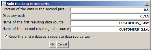
In the first input field of the dialog, we define the size ratio of the two data parts. The predefined value of 0.5 creates two parts of equal size.

The second, third and fourth Input field specify the directory path, the names and - indirectly via the file name endings - the types of the files in which the resulting partial data are to be persistently stored on disk. Leave these fields empty if you do not want to store the data parts persistently. Hence, the following alternatives are possible:

• No entry in the data name input field: the data are not stored on disk. You do not have the possibility to re-read the partial data with modified settings during the current Synop Analyzer session. If the current analyses are stored as a project and the project is reopened later, each data part must be recreated by reading the entire data and sorting out a part of it. That can consume much time on large data. On the other hand, that variant avoids the risk of unwillingly working on outdated partial data once the original data source is updated.
• An entry with ending .iad in the file name field: the data are stored on disk in the proprietary compressed iad format. That means there is no possibility to re-read the data parts with modified settings. But if the current analysis project is stored and reopened later, the data parts will be imported very fast, even if the data are large.
• An entry with ending .txt in the file name field: the data are stored on disk as flat text files. That means there is the possibility to re-read the data parts with modified settings during the current Synop Analyzer session. If the current analysis project is stored and reopened later, the data parts will be imported from the two flat files, which is faster than reading the entire original data twice, but much slower than importing two iad files.