The Regression Analysis panel
Content
Purpose and short description
Parameters for regression analsis
The Regressions result panel
Applying regression models to new data ('Scoring')
Purpose and short description
A regression analysis finds a formula which predicts the value of one single data field, the so-called target field, as a function of other data fields, the so-called predictor fields. The formula is detected during a so-called training process on data, on which both the target field and the predictor fields are filled with values. The resulting formula is also called a regression model. The regression model can later be applied to new data in which the target field values are missing in order to predict the target field values. This step is called scoring.
Synop Analyzer provides several methods for creating more general regression models, for example the neural SOM method. This chapter, however, shall be focussed on linear regression and logistic regression.
A linear regression model is a linear formula which predicts the target field value y of a numeric target field from n predictor field values x1 bis xn:
y = c0 + c1 x1 + ... + cn xn.
In logistic regression, the probability of one of the two values of a two-valued target field t (the so-called '1'-value) is expressed as a formula of the kind:
proba(t=1) = 1/(1+eb0+b1*x1+...+bn*xn).
Does every predictor field contribute exactly one regressor xi? This is only the case for numeric and Boolean data fields. More precisely, the following holds:
-
Each numeric predictor field contributes exactly one regressor xi.
-
Each non-numeric predictor field with n > 2 different values contributes n regressors, one for each field value. If the regression formula is applied to a concrete data record in order to predict the target field value, only one of these n regressors contributes its coefficient ci to the calculated result, namely the one for the field value which actually occurs in the data record.
-
For Boolean fields, we assume that the regressor for the more frequent of the two values is zero. This can always be achieved by adding its real value to the constant offset c0. The only remaining regressor for the field then captures the difference in the predicted value which results if the Boolean field does not assume its majority value but the less frequent value.
Training a linear or logistic regression model means detecting the best coefficient values ci such that the resulting formula minimizes the mean squared difference between the actual and the predicted target field values on the training data.
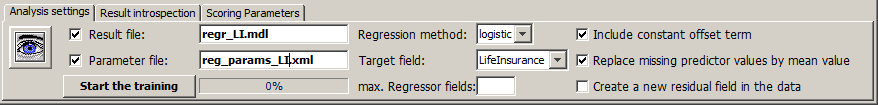
Within Synop Analyzer, a linear or logistic regression analysis is started by pressing the button  in the left screen column.
Parameters for regression analsis
The first visible tab in the toolbar at the lower end of Synop Analyzer's linear regression panel contains the available parameters for linear regression analysis.
In the following, we want to explain the process of training and interpreting a regression model at the hand of a concrete example operating on the sample doc/sample_data/customers.txt using the following settings:
-
The button
 serves to restrict the set of data fields which will be used for the model training. In our example, we do not use this feature and work with all data fields.
-
The resulting regression model will be saved under the name reg_customers.mdl in the current working directory. Per default, the created file will be a file in a proprietary binary format. But you could also save the file as a <TAB> separated flat text file, which can be opened in any text editor or spreadsheet processor such as MS Excel. Using the main menu item Preferences→Regression Preferences you can switch the output format, for example to the intervendor XML standard for data mining models, PMML.
-
The currently specified settings will automatically be saved to an XML parameter file named reg_params_customers.xml every time the button Start training will be pressed. The resulting XML file can be reloaded in a later Synop Analyzer session via the main menu item Analysis→Run regression analysis. This reproduces exactly the currently active parameter settings and data import settings.
-
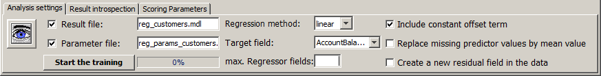
As the target field we choose the field AccountBalance. Hence, we want to create a linear regression model which is able to predict the presumable account balance, for example for new customers.
-
In the input field max. regressor fields one can limit the maximum number of predictor fields which may appear in the regression model. We do not enter a value here. If we had done it, Synop Analyzer would automatically select those predictor fields which have the maximum linear correlation with the target field.
-
In the checkbox Include constant offset term you can specify whether or not the model can contain a constant offset c0.
-
By marking the checkbox Replace missing predictor values by mean value you can modify the treatment of missing predictor field values. Per default, a missing value of a numeric predictor field is assumed as 0, that means it has no impact in the predicted target field value. If the checkbox is marked, missing values are replaced by the field's mean value when calculating the field's contribution to the target field value.
-
If the checkbox Create a new residual field in the data is marked, a new data field will be appended to the training data at the end of the training process. The new field contains the residuals, that means the differences 'actual target field value minus predicted target field value'. This information can be helpful for judging the quality and usability of the model for the intended purposes. For example, you can examine in which situation and on which data records the model delivers a good prediction accuracy and in which cases it does not.
When working with the module Linear Regression Analysis, you sometimes get the following error message:
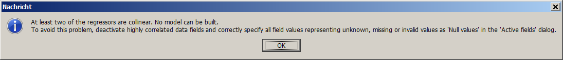
The message says that some of the predictor fields are collinear, that means perfectly correlated. In this case, no unambiguous linear regression model can be built. In the example mentioned above, the message appears due to the fact that the data field Profession contains a the value unknown on couple of data records, which all happen to have ages below 12 and the family status child. All other data records with these data subset have Profession=inactive. Therefore, the two profession values are collinear.
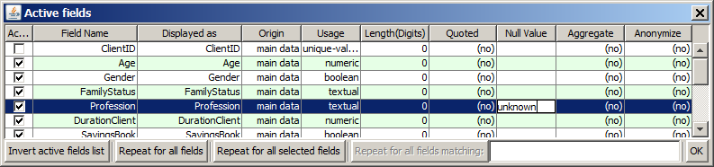
The problem can be resolved by defining the value unknown as a 'null value' for the field Profession within the pop-up dialog Active data fields before reading the data into memory. The effect of this is that the value unknown does not any more represent a valid field value, and no regressor is created for it.
The Regression result panel
After successfully terminating the training process, the main part of the window 'Regression Analysis' displays the regressors of the resulting model and their coefficients ci in the first two columns of the tabular result view.
The right column of the table ranks the corresponding predictor fields by their importance within the regression model, that means by their average impact on the predicted target field values. For calculating this impact measure, the software memorizes for each data record the contribution to the target value which comes from all regressors deriving from the one single examined predictor field. The displayed number is then the standard deviation of this list of contribution numbers.
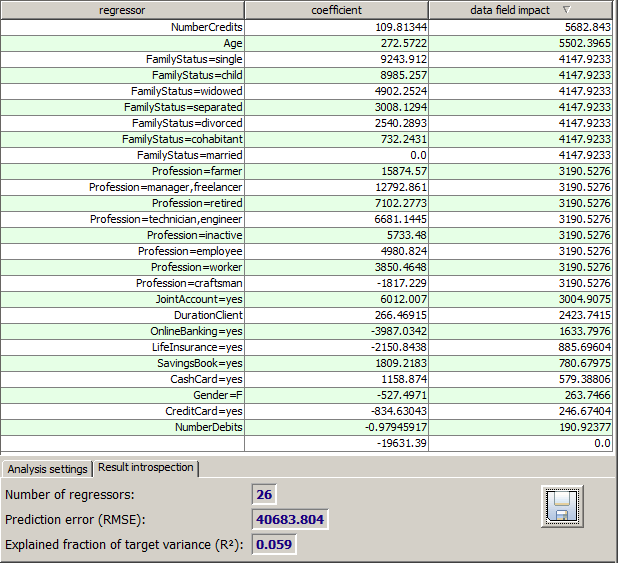
The tab Result introspection within the bottom tool bar displays the total number of regressors within the model, and it contains two quality numbers which help to judge the quality of the generated model:
-
The Prediction error (RMSE, 'root mean squared error') is the standard deviation of the residual 'actual target field value minus predicted target field value' on the training data. Hence, the value describes the mean prediction accuracy.
-
The measure Explained fraction of variance describes which fraction of the actually observed deviation of the single records' target field values from their mean value is correctly predicted by the model. A perfect model would have the value of 1, a random model, or a model which always predicts the mean target field value would have the value 0.
From the low quality values of our sample model we can see that linear regression models often deliver poor prediction quality. This is due to the fact that the linear regression approach is mathematically simple but completely neglects many important possible types of relations between the target field value and the predictor values. In particular, non-linear relations such as quadratic, exponential or cyclic relations can not be modeled, and the same holds for multi factor effects such as y = c * xi * xj.
Therefore, linear regression models should be used for actually predicting values ('scoring') with care. Rather, they are useful for studying the principal relations between different fields, and for serving as reference models for regression models created by more sophisticated algorithms such as SOM or regression trees.
Applying regression models to new data ('Scoring')
Regression models can be applied to new data in order to create predictions on these data. This application of regression models to new data for predictive purposes is called 'scoring'.
You load and apply a linear or logistic regression model by first opening and reading the new data, by then pressing the button in order to start the regression analysis module and by then clicking the button Load model in the tab Scoring Settings of the tool bar at the lower end of the panel's GUI window.
In the following sections we will demonstrate the process of regression model scoring with the help of a concrete example use case: using an logistic regression model we want to predict the propensity of newly acquired bank customers to sign a life insurance contract.
For this purpose, we load the sample data doc/sample_data/customers.txt. We keep the default data import settings with one exception but mark the field CUSTOMER_ID as the group field in the pop-up window Active Fields. Then we start the regression analysis module and train a model called regr_li.mdl, using the following parameter settings:
-
Regression method logistic,
-
Target field LifeInsurance,
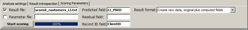
For model evaluation purposes, we apply the generated model to the training data and compare the predicted life insurance propensity to the actual existence or non-existence of a life insurance contract. In the Scoring Settings tab of the toolbar, we specify that we want to create a predicted field called LI_PRED. Optionally, we can also specify a file name to which the scoring results will be written (scored_customers_LI.txt). Then we press Start scoring in order to create the desired scoring results.
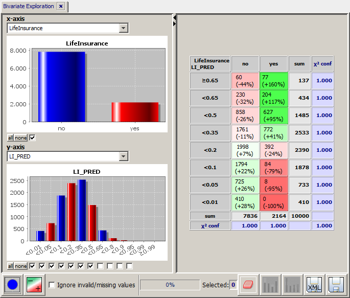
A new in-memory data source tab pops up in the left column of the Synop Analyzer workbench. In this new data source, we select the module Bivariate Exploration and select the data fields LifeInsurance as x-axis field and LI_PRED as y-axis field. The red and green colors in the bivariate matrix show us that the model's prediction generally coincides well with the actual values.
The predictions calculated on the training data could also be used for detecting interesting 'candidates' for sales actions concerning life insurance contracts. For example, one could select the customers under 50 years which do not (yet) have a life insurance but for which the model has predicted a high propensity for signing a life insurance contract:
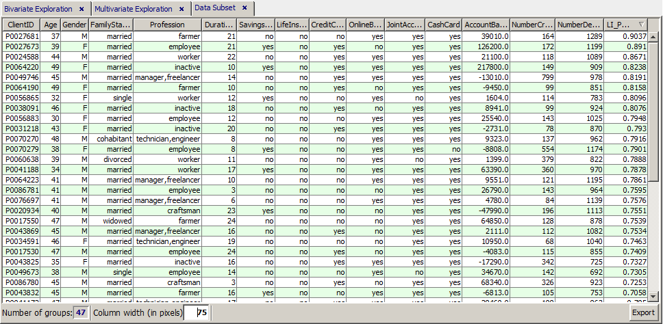
Now we apply the logistic regression model to a new data collection: 159 new customers, among which we want to find the most interesting candidates for selling life insurance contracts. We load the data doc/sample_data/newcustomers_159.txt into Synop Analyzer, thereby marking the data field CUSTOMER_ID as the 'group' field in the pop-up dialog Active fields
On this new in-memory data source, we start the regression analysis module and move to the tab Scoring Parameters in the tool bar at the lower end of the screen. Here, first load the regression model to be applied to the data, the model regr_LI.mdl. Then, we enter the name of the file in which the scoring results are to be stored (newcustomers_LI.txt), we define the scoring result data fields to be contained in that file and we specify that the new file should be a copy of the existing file newcustomers_159.txt plus the new computed data fields. (Create new data, original plus computed fields).
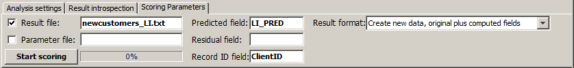
By means of the button Start scoring we create the scoring results, write the desired result file to disk and open the resulting data as a new in-memory data source in Synop Analyzer, that means as a new tab in the left column of the Synop Analyzer workbench.
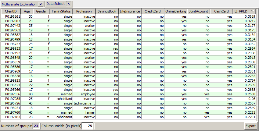
We introspect the scoring result data with the module 'multivariate exploration'. We see that the model has created a propensity probability of at least 20% for 23 of the 159 new customers whose age is below 50 years and who do not yet have a life insurance.
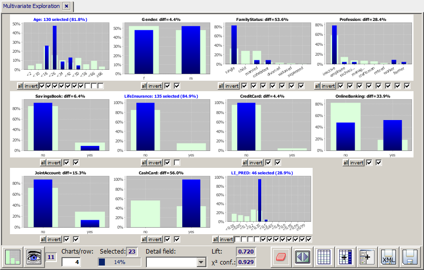
Via the button  we submit the selected 23 data records to a last visual examination. Then we can use the button Export to save the resulting list to a flat file or Excel spreadsheet, or we can use the main menu button Report to create a HTML or PDF report.