The Self-Organizing Maps (SOM) module

Content

Purpose and short description
Basic parameters for SOM trainings
Expert parameters for SOM trainings
Interpreting the result visualizations
Apply SOM models to new data
Creating scoring results

Purpose and short description

Self-organizing maps (SOM) are neural networks in which the neurons form a two-dimensional square grid or a hexagonal grid and each neuron is connected by artificial synapses to its near neighbors. A SOM is trained in an unsupervised learning process on a so-called training data set. Each neuron has a set of properties - the so-called weights - which corresponds to the set of data attributes available in the training data, and each neuron represents a unique combination of values of these attributes.

The purpose of the SOM is to define a mapping from the high-dimensional training data space with its many attribute dimensions to a two-dimensional representation which is easy to visualize and interpret but which conserves as much as possible of the structural (topological) information of the original data space.

There are two major application areas for SOM models: data visualization and data clustering on the one hand and scoring (prediction of unknown attribute values) on the other hand. In this latter case, the trained SOM model is applied to a neu data collection, the so-called scoring data, in which some of the attributes or attribute values of the original training data are missing.

You can find more details on the theoretical approach and links for further reading on http://en.wikipedia.org/wiki/Self-organizing_map.

Basic parameters for SOM trainings

In Synop Analyzer, a SOM training is started by loading a data source - the so-called training data - into memory and by clicking on the button in the input data panel on the left side of the Synop Analyzer GUI. The button opens a panel named SOM Training. In the lower part of this panel, you can specify some parameters for the next SOM training and start the training process. The training process itself can be a long-running task, therefore it is executed asynchronically in one or more parallelized background threads. After the end of the training, the resulting SOM model will be displayed in the upper part of the panel.

The following paragraphs and screenshots demonstrate the handling of the various sub-panels and buttons at hand of the sample data doc/sample_data/customers.txt. We assume that these data have been read into memory without changing any default settings in the data import panel on the left side of the screen.

The first visible tab in the toolbar at the lower end of the SOM panel contains the most important parameters for SOM trainings.

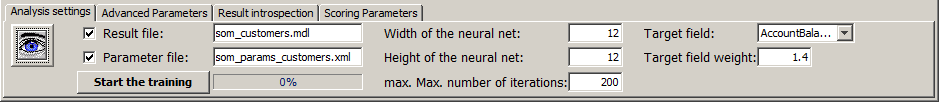
In the screenshot, the following settings were specified:

• The button serves to restrict the set of data fields which will be used for the model training. In our example, we do not use this feature.
• The trained SOM model will be saved under the name som_customers.mdl in the current working directory. Per default, the created file will be a flat file in a proprietary binary data format, which can only be opened and reused in Synop Analyzer. Using the main menu item Preferences→SOM Preferences you can switch the output format to the intervendor XML standard for data mining models, PMML.
• The currently specified settings will automatically be saved to an XML parameter file named som_params_customers.xml every time the button Start training will be pressed. The resulting XML file can be reloaded in a later Synop Analyzer session via the main menu item Analysis→Run SOM training. This reproduces exactly the currently active parameter settings and data import settings.
• The size of the neural net is set to 12 * 12 neurons, which are placed into a square grid.
• The number of training iterations during the SOM training process is limited to 200. In each iteration, the neural net learns each data record once, each data record is assigned to the neuron which best represents the properties of the data record, and then the weights (properties) of the best matching neuron itself and its nearest neighbors are shifted towards the properties of the assigned data record. This is the way the SOM net 'learns the data'. The training ends when either no further optimization of the mapping quality of the net can be reached or if the maximum number of iterations has been reached.
• When training a SOM model, one can optionally specify a target field. That means one informs the model on the fact that the model will later be used to predict this data field on new data.
• Using the parameter Target field weight you can overweight the target field relative to the other data fields when training the SOM by specifying a weight factor larger than 1. As a consequence, the resulting SOM model will fit the values of the target field particularly well, at the cost of some loss of fitting quality on the other data fields.

You should consider specifying a target weight larger than 1 if you want to train a SOM for predicting a target field and if with the default training settings the resulting SOM target field shows no clear structures but rather an amorphous green and grey pattern.

On the other hand, one can easily generate an 'over-trained' model by pushing the target weight to high. Over-training means that the resulting SOM almost perfectly maps all record's target field values but performs poorly both on the other data fields on the training data and when predicting the target field values of new scoring data.

It is always a good idea to put aside a small part of the available training before starting the SOM training. These data can then be used to validate the SOM. That means one lets the model predict the target field values and compares the predictions to the actual target field values. This approach helps to find the training parameter settings which produce the model with the smallest mean squared difference between the actual and the predicted target field values.

Expert parameters for SOM trainings

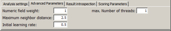
The second tab at the lower end of the screen, Advanced Parameters, provides 4 parameters which serve for fine-tuning the training process. You should only modify them if you are familiar with the SOM approach and algorithm parameters such as 'learning rate' or 'neighborhood radius'.

• Numeric field weight: Per default, each numeric data field contributes with the same weight factor (of 1) to the distance calculations between neurons and data records as the Boolean and textual fields. You can define a higher or lower weight factor for the numeric fields compared to Boolean and textual fields using this parameter. Note that weight settings for specific fields, for example the target field weight, overwrite this general setting, the weight factors are not multiplied.
• The maximum neighbor distance is the Euclidean distance (dx² + dy²) between neurons up to which learned information is distributed from the best matching neuron to neighbored neurons of that neuron. If that value is 1.5, for example, then 8 neighbored neurons are influenced by each assignment of a data record to its best matching neuron, namely the neuron's 4 nearest neighbors at distance 1 and 4 second nearest neighbors at distance 1.41. During the SOM training process, the maximum neighbor distance is reduced step by step.
• The initial learning rate is the strength of change of a neuron's properties when a new data record is being learned. If the learning rate is 0.5, for example, and if the best matching neuron of a data record with Age=46 has the property Age=40 before learning the record, the neuron's property will have changed to Age=43 after learning the data record.
• The parameter max. number of threads specifies an upper limit for the number of parallel threads started by the SOM training engine in order to perform the training. If this input fields contains a value of 0 or smaller, the software is free to fully exploit the available CPU, that means to start one thread on each CPU core of the computer.

Interpreting the result visualizations

The third tab within the tool bar at the lower border of the SOM training window offers some capabilites to modify the display mode of the created SOM model and to introspect and export the model itself or certain data clusters marked on it. Some of the buttons only become enabled if you have selected one or more neurons by mouse clicks within the SOM cards.

The screenshot shown below results if one performs the parameter settings described in the previous sections and then presses the button Start training.

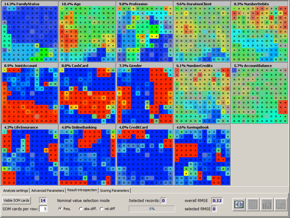
The main part of the screen displays one separate map, a so-called SOM card, for each data field. The SOM cards can be interpreted as follows:

• The title row of each card shows the name of the data field which the card describes as well as an importance percentage number which indicates how important the data field is for the SOM model. The sum of all importance numbers is always 100%. A high value indicates that the SOM model is able to predict the values of this data field on almost all training data records with high accuracy and confidence and that the SOM card shows a clear structure of large and homogeneous regions. Small importance numbers result from SOM cards which look like rag rugs of which have many grey spots, which indicates that the data records mapped to these neurons have a rather diffuse value range,
• Each single small uniformly colored squaree within a SOM card represents one neuron. Hence, all SOM cards in our example consist of 12 * 12 small colored squares.
• The black dots or black quadrangles in the center of each colored square indicate how many training data records have been mapped to this neuron. A small dot represents one single data record or a very small number of data records, the longer each side of the quadrangle is, the more data records have been mapped to the neuron. You can hide this additional information by right-clicking on one of the SOM cards while keeping the <Ctrl> key pressed.
• The color coding scheme of the SOM cards representing numeric data fields correspond to the familiar color coding of topographical maps: low values are blue, medium values green and high values red.
• In the SOM cards for textual data fields, for example in the card for the field FamilyStatus in our example, the most frequent value (married) is dark blue, the second most frequent value light blue, the third one turquoise, and so on through the rainbow. The least frequent field values are orange or red.
• In the SOM cards for Boolean, that means two-valued fields such as the field Gender, the majority value is blue, the minority value red.
• The intensity of each colored square indicates how precisely and reliably the data field values of the training data records mapped to the neuron represented by the square coincide with the neuron's own value for the data field. The more precise and reliable the mapping, the higher the intensity. If the square is gray then the data records mapped to the neuron have a standard deviation or value distribution which is as diffuse as on the entire training data.

Synop Analyzer's SOM cards provide a wide variety of mouse-based interactivity and selection features:

• By left-clicking one of the colored squares in one of the SOM cards, the corresponding neuron is selected on all visible SOM cards. The title information of each SOM card changes and shows the statistical properties of the training data records which have been mapped to the selected neuron. Additionally, the bottom tool bar shows the absolute and relative number of data records mapped to the selected neuron. In the picture shown above, a neuron in the middle of the second row from the top of the SOM card has been selected.
• Left-clicking a colored square while keeping the <Ctrl> key pressed adds a new selected neuron to the current selection. That means, you can select more than one neuron at once.
• Left-clicking a colored square while keeping the <Shift> key pressed selected large regions of neurons at once. More precisely, the click starts a 'flooding' algorithm which selects all neurons starting from the current position in every direction until the end of the SOM card is reached or an already selected neuron is reached.
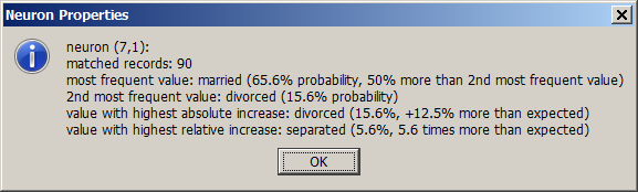
• Right-clicking a colored square within a SOM card opens a pop-up dialog in which the statistical properties of the neuron and the training data mapped to it are shown in detail.
  For numeric data fields, the pop-up window shows the mean and standard deviation of the data field values of all training data records mapped to the neuron.
  
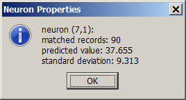
  For textual data fields, the pop-up window shows the most frequent value with its percentage of occurrence, and the values which have the greatest increase rate on the neuron compared to the entire training data. There are two increase rates: an absolute or additive one (the added percentage rate), and a relative or multiplicative one (the multiplication factor of occurrence probability):
  
  
• Right-clicking a square while keeping the <Ctrl> key pressed switches the additional occupation frequency information, that means the black dots and quadrangles, on or off

In the tool bar tab Result introspection, the following options are available:

• The button Visible SOM cards opens a pop-up dialog in which you can restrict the set of data fields whose SOM cards are to be shown on screen. The blue number at the right side of the button displays the number of currently visible SOM cards.
• The input field SOM cards per row specifies how many SOM cards will be shown within one screen row. Hence, the field defines how big each single SOM card will appear on screen.
• The three radio button labeled Nominal value selection mode permit to switch between three display modes within the SOM cards for textual data fields. The default mode is shown on the left side of the picture below. In this mode, each square (neuron) is colored according to the most frequently adopted field value on all training data records mapped to this neuron, independent from the fact whether or not this value's occurrence rate is greater or smaller than the value's occurrence rate on the entire training data. In the neuron selected in the picture below, this majority value is the value married with an occurrence rate of 65.6%.
  
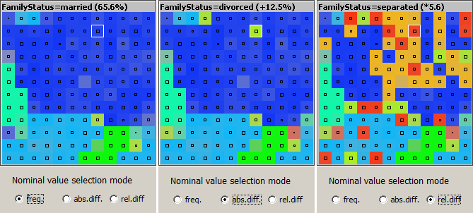
  In the display mode Absolute difference, the neuron is colored like the value which has the highest absolute (additive) increase rate on the neuron compared to the entire data. That can but need not be the majority value. In our example, it is the value divorced, which has an occurrence rate of 15.6% on the neuron, hence an increase of 12.5 percent points compared to its overall occurrence rate of 3.1%.
  In the third display mode Relative difference, the neuron is colored like the value which has the highest relative (multiplicative) increase factor on the neuron compared to the entire training data. In our example, it is the value separated. This value occurs 5.6 times more probably on the data records mapped to the neuron than on the entire data, where it occurs in only 1% of all data records.
  From the picture shown above it becomes visible that the first display mode favors the most frequent field values, in the second mode also moderately frequent values have a chance to appear, and in the third mode the least frequent values are favorized because it is easier to reach high multiplication factors of occurrence when starting from a small base.
• The output field Selected records and the percentage bar displayed below the field show the absolute and relative size of the data subset which has been mapped to the currently selected neurons.
• The output field Overall RMSE contains a measure for the average accuracy of the mapping induced by the SOM, that means the mapping from the n-dimensional input data space to the two-dimensional neural network. RMSE stands for root mean squared error, that is the square root of the average over the squared mapping errors, where the squared mapping error between a neuron an a data record is the average over all squared differences between the neuron's value for each data field and the field's value on the data record. RMSE is scaled such that a value of 1 corresponds to a useless or trivial SOM model in which all neurons have identical properties: the adopt the field's mean value for numeric fields and they adopt a value occurrence distribution equal to the overall distribution on the training data for the non-numeric fields. A value of 0 stands for a perfect SOM which has no mapping error at all.
• The output field Selection RMSE contains the corresponding measure to overall RMSE for the subset of the training data which has been mapped to the currently selected neurons.
• By clicking on this button you re-draw all SOM cards, thereby adapting their size to the current screen width.
• opens a new panel which contains the data records which have been mapped to the currently selected neurons in tabular form. In the panel, you can sort the selected data by any data field and export the extire selection or a subset into a flat file or spreadsheet.
• opens an additional window in which the data groups mapped to the currently selected neurons can be visually explored. (See picture below.)
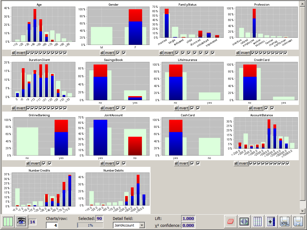
  The new window provides the entire functionality of the module multivariate analysis. The screenshot shown below explores the 90 data groups which have been mapped to the neuron which has been taken as our example selection in the previous pictures. Additionally, we have chosen the data field JointAccount as detail structure field. Now the blue and red bars are indicating how the dagree of usage of a joint account coincides with age, family status, account balance etc. on the selected customers.
• Using the button you can export the data groups mapped to the currently selected neurons into a <TAB> separated flat text file or into a spreadsheet in .xlsx format.

Apply SOM models to new data

SOM models which have been trained and stored earlier can later be reloaded and applied to a new data source. Synop Analyzer then compares the data fields available in the new data and the data fields used in the SOM model. Applying the model to the new data is only possible if at least half of the data fields used in the model are available in the new data. You load and apply a SOM model by first opening and reading the new data, by then pressing the button in order to start the SOM module and by then clicking the button Load model in the fourth tab of the tool bar at the lower end of the SOM panel's GUI window.

Once the SOM model has been loaded and applied successfully, the same SOM cards appear that you have seen at the end of the training process on the training data. But the black dots and quadrangles within the cards now represent the mapping of the new data records to the neural net. Correspondingly, the mapping quality measures Overall RMSE and Selection RMSE as well as the displayed relative and absolute numbers of selected data records shown in the panel's bottom tool bar now refer to the new data.

When applying a SOM model to a new data source, you should always have a look at the measure Overall RMSE. If this value is much larger on the new data than it was on the training data, the new data do not match the model very well, indicating that between the training data and the application data, some major shift in the rules and relations which interrelate the different data fields and their values has occurred. Hence, using this SOM model for scoring the new data, that means for predicting missing field values, can yield misleading results.

In our example, we see from the distribution of the black quadrangles that the average demographic properties of the new customers do not coincide with the average demographic proberties of the existing customer base - new customers are mostly children or young adults. But nontheless, the model seems well applicable to the new data because the overall RMSE value is only slightly larger than it was on the training data, and it is still close to 0.

Creating scoring results

Now we want to use the loaded SOM model for scoring, more precisely for predicting the average account balance that we can expect from each new customer after a few months of getting into business with him or her. This information can be important for customer relationship management aspects and for optimizing the bank's internal refinancing strategy. The tab Scoring Settings within the SOM panel's bottom tool bar offers the following customization parameters for the SOM scoring:

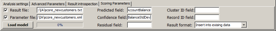
• Using the input field Result file you can enter the name of a flat file into which the scoring result data are to be written.
• Analogously, you can specify the name of an XML file which will persistently store the current SOM settings using the input field Parameter file.
• The button which previously showed the label Load model now displays the text Start scoring. By pressing this button, you start the scoring process after entering all desired customization settings.
• The next five input fields serve to define the names of computed data fields which will be added to the data and which will contain different scoring results. Normally, you are interested in only two or three of the available scoring results, then you should leave the other field names empty. The five different possible scoring result fields are the following:
  • Predicted field is the name of the data field into which the predicted values of the field will be written which has been specified as the target field when the SOM model was trained. In our case, the model's target field was Kontensaldo; in the new data, a field with this name is missing, therefore we choose exactly this name for the predicted field.
  • Confidence field is the name of the data field into which the model's self-estimation of the accuracy of each record's target field prediction will be written. If the target field is numeric, the confidence field will contain the estimated mean prediction error (standard deviation). For textual target fields, the confidence field will contain the estimated probability that the predicted value is the correct one. In our example, we are interested in this information and call the field BalanceStdDev.
  • Residual field is the name of the data field into which the difference between the predicted and the actual target field value will be written. Activating this field only makes sense on validation data which already contain target field values before the scoring and on which the scoring is started for model validation purposes. Therefore, we leave the field name empty in our example.
  • SegmentID field is the name of the data field into which for each data record the number of the best matching neuron will be written. This field is only of interest of the SOM scoring is started with the aim of clustering the data. This is not the case in our example, therefore we leave the field empty.
  • RecordID field is the name of the data field into which the SOM scoring engine will write the group field value of each scored data record, or, if no group field has been defined, a record ID running from 1 to the number of records in the application data. This field is important if the scoring results are to be written into a completely new data file and not to be merged into the existing data. In the first case, one normally needs a sort of primary key in the newly created data file for later being able to combine and join the new data with existing data sources. In our example write the scoring results directly into the existing data, therefore we do not need this field.
• The last selection field in the tab, Result format, specifies whether the newly created scoring results are to be merged into the existing data or written into a completely new data file, and if the latter is the case, whether the new file shall only contain the newly computed scoring result fields or also the preexisting data fields of the application data.

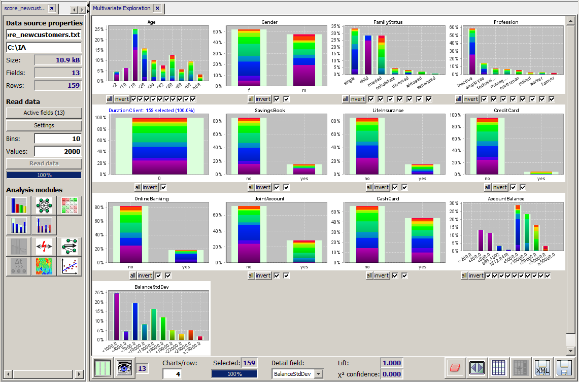
We have selected the new data field BalanceStdDev as the detail structure field of our visualization. This field contains the SOM model's self-estimation on the accuracy of each of its predictions. Blue or violett values correspond to low incertitude ranges, orange and red values to very high incertitude ranges. For some data records, the SOM thought that its prediction was very accurate - up to some 100 EUR - for other data records the model gave an incertitude range of up to 30,000 EUR.

In our example we understand that the average balance of children can be predicted quite precisely and that surprisingly the self-estimated prediction quality for men is more often very low or very high than for women, where medium incertitude ranges dominate.

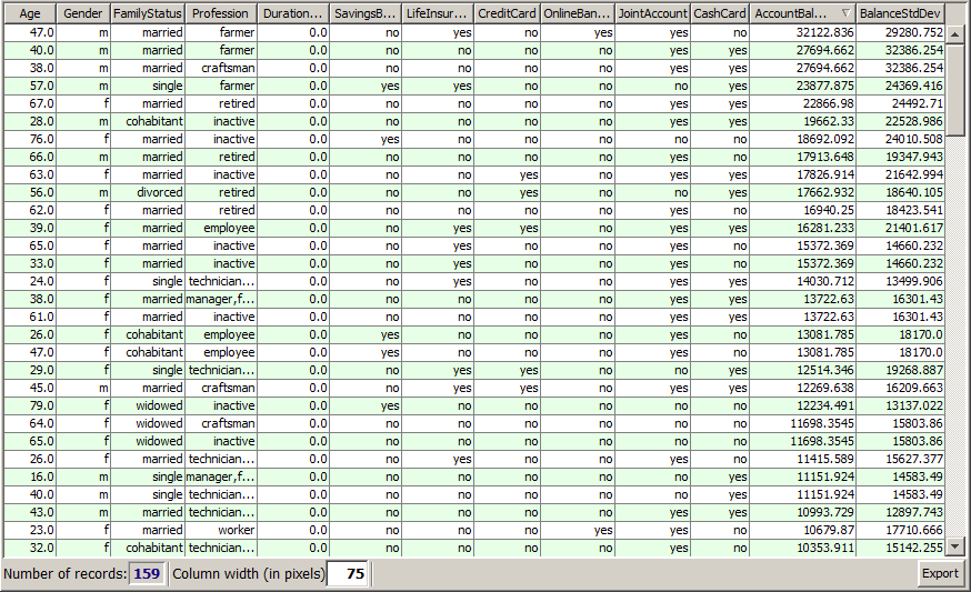
By pressing the button one can introspect the entire scoring results in tabular form, sort and filter them and export parts or all of them into different persistent target formats such as flat text files or spreadsheets. In the picture shown below we have sorted the scoring results by decreasing predicted value. We see that the model predicts the highest account balances for 40 to 55 years old engineers, freelancers, craftsmen and farmers and for pensioners.