The Associations Analysis module
Content
Purpose and short description
Input data formats
Definitions and notations
Basic parameters for an associations analysis
Pattern content constraints ('item filters')
Pattern statistics constraints ('numeric filters')
Result display options
Pattern verification and significance assurance
Applying association models to new data ('Scoring')
Purpose and short description
An associations analysis finds items in your data that are associated with each other in a meaningful way. Within Synop Analyzer, an associations analysis is started by pressing the button  in the left screen column.
An item is an 'atomic' piece of information contained in the input data, that means a combination of a data field name and a field value, for example PROFESSION=farmer. A prerequisite for finding associations between these atomic items is that a grouping of several of the items to one comprising group of data fields or data records exists. Often, this group of fields or records is called a transaction (TA).
An association is a combination of several items, a so-called item set, for example the combination PROFESSION=farmer & GENDER=male. An association rule is a combination of two item sets in the form of a rule itemset1 → itemset2. The left hand side of the rule is called the rule body or antecedent, the right hand side the rule head or consequent.
The table below lists typical use cases for associations analysis [Ballard, Rollins, Dorneich et al., Dynamic Warehousing: Data Mining made easy]:
| industry | use case | grouping criterion | typical body item | typical head item |
| retail | market basket analysis | bill ID or purchase ID | a purchased article | another purchased article |
| manufacturing | quality assurance | product (e.g. vehicle ID) | component, production condition | problem, error ID |
| medicine | medical study evaluation | patient or test person | single treatment info | medical impact |
Input data formats
Synop Analyzer's association detection module is prepared for working with three different data formats:
-
The transactional or pivoted data format:
Often, the input data for associations mining are available in a format in which one column is the so-called group field and contains transaction IDs, one or more additional fields are the so-called item fields and contain items, i.e. the information on which associations are to be detected.
Synop Analyzer expects that data with a group field are sorted by group field values. If the data are read from a database, Synop Analyzer automatically assures that property by issuing a SELECT statement with an appropriate ORDER BY clause. If the data are read from flat file or from a spreadsheet, the user is responsible for bringing the data into the correct order. Synop Analyzer will issue a warning message if the data are not correctly ordered.
The file doc/sample_data/RETAIL_PURCHASES.txt is an example for such a data format: the field PURCHASE_ID is the group field, the field ARTICLE contains the real information, namely the IDs of the purchased articles.
In the transactional data format, the items appearing in the detected association patterns are a combination of field name and field value if there is more than one item field; the name of the item field is omitted if all items come from one single field (such as the field ARTICLE).
-
The data format with Boolean fields:
You can also detect associations on input data which do not have a group field (that means each data row represents a separate transaction) and in which each single 'item', i.e. each single event or fact, has its own two-valued (Boolean) data field which indicates whether or not the item occurs in the transaction.
If the field PURCHASE_ID was missing in the sample data doc/sample_data/RETAIL_PURCHASES.txt and if there was a separate data field for each existing article ID which contained either 0 or 1, depending on whether or not the corresponding article was purchased in transaction represented by the current data row, then the data would have the data format with Boolean fields.
If Synop Analyzer detects a data format with Boolean fields, it interprets all Boolean field values starting with '0', '-', 'F' or 'f' (such as 'false'), 'N' or 'n' (such as 'no' or 'n/a') as indicators for 'item does not occur in the transaction', all other values are interpreted as 'item occurs in the transaction'.
In the data format with Boolean fields the items appearing in the detected association patterns contain only the names of the Boolean fields, but not the field values such as 'YES' or '1'.
-
The 'normal' or broad data format:
Of course, Synop Analyzer can also detect associations on 'normal' data in which each single data row is considered one data group and in which there are different data fields of various types which contain the items. doc/sample_data/customers.txt is an example for such a file.
On these data, the items appearing in the detected patterns always have the form 'field_name=field_ value'.
A general rule, which is valid on all data formats, is: the items which form the detected associations can only come from active data fields which have not been marked as 'group', 'entity', 'oder' or 'weight'. 'entity' fields are ignored in associations mining (they are only important for sequential patterns analysis), 'group' field values serve to define data groups covering more than one data row, information from 'order' fields is used to calculate trend coefficients for the detected associations, and information from 'weight' fields is used to calculate pattern weight coefficients.
Definitions and notations
An association pattern or rule can be characterized by the following properties: [Ballard, Rollins, Dorneich et al., Dynamic Warehousing: Data Mining made easy]
-
The items
which are contained in the rule body, in the rule head, or in the entire rule.
-
Categories of the contained items.
Often, an additional hierarchy or taxonomy for the items is known. For example, the items 'milk' and 'baby food' might belong to the category 'food', 'diapers' might belong to the category 'non-food'. 'axles=17-B' and 'engine=AX-Turbo 2.3' might be members of the category 'component', 'production_chain=3' of category 'production condition', and 'delay > 2 hours' of category 'error state'. Hence, the second sample rule can be characterized by the fact that its body contains components or production conditions, and its head an error state.
-
The support of the pattern:
Absolute support S is defined as the total number of data groups (transactions) for which the rule holds. Support or relative support s is the fraction of all transactions for which the rule holds.
-
The confidence of the pattern when interpreted as a rule:
Confidence C is defined as
C := s(body & head) / s(body).
-
The lift of the pattern:
The Lift L of a pattern Item1 & ... & Itemn is defined as
L := s(Item1 & ... & Itemn) / (s(Item1) * ... * s(Itemn)).
lift > 1 (< 1) means that the pattern appears more (less) frequently than expected assuming that all involved items are statistically independent.
-
The rule lift of the pattern when interpreted as a rule:
The rule lift Lr is defined as
Lr := s(body & head) / (s(body) * s(head)).
Lr > 1 (< 1) means that the pattern body & head appears more (less) frequently than expected assuming that body and head are statistically independent.
-
The purity of the pattern:
The purity P of a pattern Item1 & ... & Itemn is defined as
P := s(Item1 & ... & Itemn) / maxi=1...n( s(Itemi) ).
P = 1 means that the pattern describes a 'perfect tupel': none of the items Itemi ever occurs without all the other items in the same data group.
-
The core purity of the pattern:
The core purity Pc of a pattern Item1 & ... & Itemn is defined as
Pc := s(Item1 & ... & Itemn) / mini=1...n( s(Itemi) ).
Pc = 1 means that at least one of the items involved in the pattern does never occur in the data without the n-1 other items of the pattern. An item with this property is called a 'core item' of the pattern.
-
The weight (cost,price) of the pattern:
If a weight field has been defined on the input data, we can calculate the average weight of the data groups which support the pattern. If, for example, in those purchases which contain the items 'milk', 'baby food' and 'diapers', the mean overall purchase value is 49.69$, the weight of the pattern (milk & baby food & diapers), and also the weight of the corresponding association rule (milk & baby food) → diapers , is 49.69$.
-
The χ2 confidence of the pattern:
The χ2 confidence level of an association indicates up to which extent each single item is relevant for the association because its occurrence probability together with the other items of the association significantly differs from its overall occurrence probability.
More formally, the χ2 confidence level is the result of performing n χ2 tests, one for each item of the association. The null hypothesis for each test is: the occurrence frequency of the item is independent of the occurrence of the item set formed by the other n-1 items.
Each of the n tests returns a confidence level (probability) with which the null hypothesis is rejected, and the χ2 confidence level of the association is set to the minimum of these n rejection confidences.
Basic parameters for an Associations analysis
In Synop Analyzer, an associations analysis is started by loading a data source - the so-called training data - into memory and by clicking on the button in the input data panel on the left side of the Synop Analyzer GUI. The button opens a panel named Associations Detection. In the lower part of this panel, you can specify the settings for an associations analysis and start the search. The detection process itself can be a long-running task, therefore it is executed asynchronically in several parallelized background threads. In the upper part of the panel, the detected association rules - the so-called association model - are displayed.
The following paragraphs and screenshots demonstrate the handling of the various sub-panels and buttons at hand of the sample data doc/sample_data/customers.txt.
The first visible tab in the toolbar at the lower end of the screen contains the most important parameters for associations analysis.
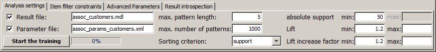
In the screenshot, the following settings were specified:
-
The detected association patterns will be saved under the name assoc_customers.mdl in the current working directory. Per default, the created file will be a file in a proprietary binary format. But you could also save the file as a <TAB> separated flat text file, which can be opened in any text editor or spreadsheet processor such as MS Excel. Using the main menu item Preferences→Associations Preferences you can switch the output format, for example to the intervendor XML standard for data mining models, PMML.
-
The currently specified settings will automatically be saved to an XML parameter file named assoc_params_customers.xml every time the button Start training will be pressed. The resulting XML file can be reloaded in a later Synop Analyzer session via the main menu item Analysis→Run associations analysis. This reproduces exactly the currently active parameter settings and data import settings.
-
The patterns to be detected should consist of up to 5 parts (items). When specifying the parameters for an associations training, you should always specify an upper boundary for the desired association lengths, otherwise the training can take extremely long time.
-
The upper limit for the number of patterns to be detected and displayed is set to 1000. If more patterns are found, the 1000 patterns with the highest values of the measure currently specified in the selector box Sorting criterion will be selected. In our example, the 1000 patterns with highest support will be selected.
-
The patterns to be detected should occur in at least 50 data groups (transactions). When specifying the parameters for an associations training, you should always specify an lower boundary for the absolute or relative support, otherwise the training can take extremely long time.
-
Only patterns whose lift is at least 1.2 are to be detected. Hence, we are interested only in 'frequent' patterns which appear on at least 20% more data groups than it could have been expected from the frequencies of the involved items.
-
The patterns consisting of more than two parts (items) must have lift increase factors of at least 1.2. An association pattern of n > 2 items has n lift increase factors, namely the patterns own lift value divided by the n lift values of the n 'parent' patterns in which exactly one of the n items is missing.
The specification of an upper or lower limit for the lift increase factor often is a very effective means for preventing the set of detected patterns from growing too big and for suppressing the appearance of 'redundant', trivial extensions of relevant patterns by just appending arbitrary items to them. As a general rule, one should always specify a minimum value larger than 1 for both lift and lift increase factor if one is looking for typical, frequent patterns. On the other hand, if one is looking for deviations, one should always specify a maximum lift and maximum lift increase factor smaller than 1.
Pattern content constraints ('item filters')
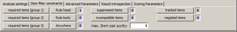
Filter criteria defining the desired contant of the patterns to be detected can be specified using the second tab named Item filters of the bottom part of the associations analysis screen. The tab itself displays how many content filter criteria of the various types have been set, the specification of new content filter criteria is performed within pop-up dialogs which open up when one presses one of the buttons in the tab.
-
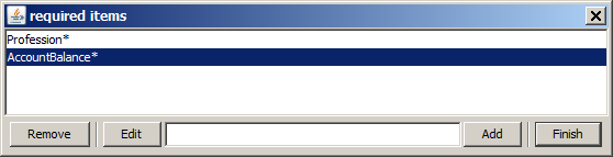
The three buttons named Required items (group n) define items which must occur in each detected pattern. If several item patterns are specified within one 'required group', at least one of them must appear in each detected association. In the Associations analysis module, up to 3 different groups of required items can be specified. The detected patterns must contain at least one item out of every specified group.
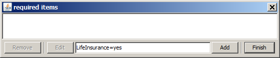
Each item specification can contain wildcards (*) at the beginning, in the middle and/or at the end. A wildcard stands for an arbitrary number of arbitrary characters or nothing. The spelling of the items with upper case and lower case letters and empty spaces must exactly match the spelling of the field names and value names as it is displayed in the module . You can either type in the desired values into the input field, or you can select one or more values from a drop-down list of all available items in the data by pressing the arrow symbol at the right edge of the input field.
As the first required item group we specify 'LifeInsurance=yes'. That means we look for patterns which have something to do with the fact that a customer has a life insurance contract with the analyzed bank. We enter the text into the editor field of the pop-up dialog and then press Add.
-
As the second required group we specify
Profession* and AccountBalance*. That means, we enforce that each detected patterns contains an information either on the profession or on the account balance of the customer.
-
The buttens at the left of the three 'required item' buttons specify allowed positions of the required items within the association rules to be detected. Anywhere means that the item may occur anywhere within the rule, Rule body means that the item must occur on the left side ('if') of the rule, Rule head means that the item must occur on the right side ('then') of the rule.
-
Suppressed Items are items which are to be ignored during the pattern search. In our example, we are not interested in any information on joint accounts, therefore we enter
Join* into the pop-up dialog suppressed items.
-
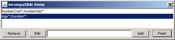
If a pair of items or item groups has been specified as incompatible (by pairs), then none of the detected associations will contain more than one item out of this set. In the text field of the pop-up dialog, you can enter several patterns, separated by comma (,) without adjacent spaces. If a pattern contains a comma as part of the pattern name, escape it by a backslash (\). Each pattern can contain one or more wildcards (*) at the beginning, in the middle and/or at the end.
In general it is reasonable to specify items from highly correlated data fields as 'incompatible'. Otherwise one would obtain many patterns with very high lift values in which one item from each of the two highly correlated fields appears. These trivial associations might shadow the truely interesting, non-trivial associations.
In our example, we define the item pairs NumberCredits and NumberDebits as well as the pairs Age and DurationClient as incompatible.
-
The item pair purity of two items i1 and i2, is the number of transactions in which both items occur divided by the maximum of the absolute supports of the two items. Item pairs with a purity of 1 are 'perfect pairs': whenever i1 occurs in a transaction, also i2 occurs in it, and vice versa.
Defining an upper limit for the permitted item pair purity is therefore an alternative means for specifying many single incompatible item pairs. It serves to suppress all trivially highly correlated item pairs from the associations analysis.
In our example, we have suppressed all item pairs which have a purity of 0.75 (75%) or more.
-
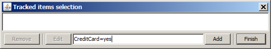
Tracked items are items whose occurrence rate is tracked and shown for every detected association. The tracked rate indicates the probability that the tracked item occurs in a data record or group which supports the current association.
In our example, we specify that we want to be shown the percentage of credit card users on the support of every single pattern that will be detected.
-
Negative items are items for which the complement, i.e. the fact that the item does NOT occur, should be treated as a separate item. For example, if the item 'OCCUPATION=Manager' is added to the list of negative items, then the item '!(OCCUPATION=Manager)' is created, and its support is the complement of the support of 'OCCUPATION=Manager'.
In our example, we specify the item Profession=inactive as negative item. That means, we want the fact that a customer has a profession to appear as a new item in the detected patterns.
Advanced pattern statistics constraints
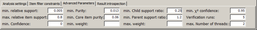
The third tab at the lower end of the screen, Advanced Parameters, provides 12 parameters which serve for fine-tuning the detected pattern set based on certain statistical measures.
-
The relative support of the patterns to be detected in our example must be at least 0.005, or 0.5%. When specifying the parameters for an associations training, you should always specify an lower boundary for the absolute or relative support, otherwise the training can take extremely long time. In our example, however, setting the minimum relative support to 0.005 has no real effect and is redundant since we have already specified a minimum absolute support of 50, and there are about 10000 data groups in the sample data.
-
The relative support of an item is the item's absolute support divided by the total number of transaction (groups). In other words, the relative support is the a-priori probability that the item occurs in a randomly selected transaction. Items which appear in (almost) every data group often represent trivial information which one does not want to find in the detected patterns. In our example, we have specified an upper boundary of 0.8 in order to suppress items which occur on at least 80% of all transactions.
-
The confidence of an association rule is the ratio between the rule's support and the rule body's support. An association rule is an association of n items in which n-1 of the n items are considered the 'rule body' and the remaining item is considered the 'rule head'. Hence, n different association rules can be constructed from one association of length n. A rule's confidence is the probability that the rule head is true if one knows for sure that the rule body is true. In our example we have specified that we want to search only those associations in which the confidence of at least one possible split into body and head yields a confidence value of at least 0.2.
-
The purity of an association is the ratio between the association's support and the support of the most frequent item within the association. In our example, we have specified a minimum required purity of 0.013, that means we accept patterns whose items appear much more frequently than the entire pattern.
-
The core purity of an association is the ratio between the association's support and the support of the least frequent item within the association. In our example, we have specified a minimum required purity of 0.013, that means we accept patterns in which even the least frequent item appears much more frequently than the entire pattern.
-
The weight of an association is the mean weight of all data groups which support the association. A minimum or maximum threshold for the associations' weights can only be specified if a weight field has been defined on the input data. Therefore, we leave the two input fields for minimum and maximum weight empty.
-
The parameter minimum child support ratio defines boundary for the acceptable 'support shrinking rate' when creating expanded associations out of existing associations. An expanded association of n items will be rejected if at least one of the n parent associations has a support which is so large that when multiplied with the minimum shrinking rate, the result is larger than the actual support of the expanded association. In our example we have specified the value of 0.25. That means we suppress the formation of patterns whose support is less than 25% of the support of the least frequent parent pattern.
-
Minimum Parent support ratio is the acceptable support growth when comparing a given association to its parent associations. A parent association (of n-1 items) will be rejected if its support is less than the support of the current association (of n items) multiplied by the minimum parent support ratio. The effect of this filter criterion is that it reduces the number of detected associations by removing all sub-patterns of long associations whenever the sub-patterns have a support which is not strongly larger than the support of the long association. Inour example, we have set a value of 1.2. That means, parent patterns will be eliminated from the result set whenever their support is less than 120% of the supports of any of their longer child patterns.
-
The χ2 confidence level of an association indicates up to which extent each single item is relevant for the association because its occurrence probability together with the other items of the association significantly differs from its overall occurrence probability.<p> More formally, theχ2 confidence level is the result of performing n χ2 tests, one for each item of the association. The null hypothesis for each test is: the occurrence frequency of the item is independent of the occurrence of the item set formed by the other n-1 items.<p> Each of the n tests returns a confidence level (probability) with which the null hypothesis is rejected, and the χ2 confidence level of the association is set to the minimum of these n rejection confidences.
-
Verification runs serve to assess whether the detected association or sequential patterns are statistically significant patterns or just random fluctuations (white noise). For each verification run, a separate data base is used. Each data base is generated from the original data by randomly assigning each data field's values to another data row index within the same data field. This approach is called a permutation test. The effect is that correlations and interrelations between different data fields are completely removed from the data.
If one finds association or sequential patterns on a permuted data base, one can be sure that one has detected nothing but noise. One can record and trace the measure tuples (pattern length, support, lift, purity) of all detected noise patterns. The edge of the resulting point cloud defines the intrinsic 'noise level' of the original data. Patterns detected on the original data can only be considered significant if their corresponding measure triples are well above the noise level.
-
The parameter maximum number of threads specifies an upper limit for the number of parallel threads used for reading and compressing the data. If no number or a number smaller than 1 is given here, the maximum available number of CPU cores will be used in parallel.
Result display options
The fourth tab within the tool bar at the lower border of the associations analysis window offers some capabilites to modify the display mode of the detected associations and to introspect and export them. Some of the buttons only become enabled if you have selected one or more patterns by mouse clicks in the result table above the tool bar.
The screenshot shown below results if one performs the parameter settings described in the previous sections, presses the button Start training in the first tab and finally selects one of the resulting patterns by left mouse click.
The tabular view of detected patterns contains the statistical measures of each pattern and its content, the items which form the pattern. The most important statistical measures are, from left to right: the number of items in the pattern, the pattern's absolute and relative support, the absolute supports of the involved items, the lift, purity and core item purity, and finally the list of the items which form the pattern.
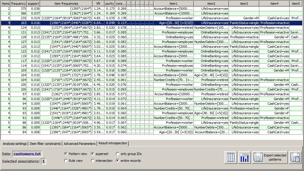
The items describing numeric data field values contain, in addition to the value range limits, an extra information within curly braces: the position of the value range within the overall value distribution of the numeric data field. For example, the item Age=[20..30[ {=3(10)} means that the age range from 20 (incl.) to 30 (excl.) is the third smallest out of 10 value ranges, hence the age value is below average but not strongly below average.
The numbers in the table column item frequencies contain the absolute supports of the different items of the pattern, in the same order in which the item names appear in the columns at the right end of the result table. If the number is marked by a star (*), the corresponding item belongs to the core of the pattern. That means that each partial pattern in which this item has been removed has a larger support than the original pattern.
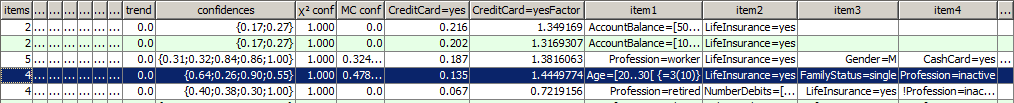
The tabular result view also contains some more advanced information on the detected patterns. In the figure shown below these columns have been enlarged and thus highlighted:
-
The measure trend indicates whether an association pattern has become more important recently (value > 0) or less important (value < 0). The measure can only be computed if an order field (time stamp field) has been defined on the input data. If an oder field exists, the trend number is calculated from a histogram of the order field as it is displayed in the module Multivariate Exploration. This is done by comparing the value distribution of the order field on the data groups which support the given pattern to the corresponding value distribution on the entire data.
More familiarly spoken: if the blue bars are higher than the light green bars on the right side of the histogram, the trend value is positive, if they are smaller than the light green bars, the value is negative. More precisely, the displayed trend value is computed out of three contributions: a 'long-term' point of view which compares the two series of bars on all N available order field value ranges, a 'short-term' point of view which compares the two series on the last 5 available data points, and a 'mid-term' point of view which compares the two series on the last M time points, where M is the geometrical mean of 5 and N.
More familiarly spoken: if the blue bars are higher than the light green bars on the right side of the histogram, the trend value is positive, if they are smaller than the light green bars, the value is negative. More precisely, the displayed trend value is computed out of three contributions: a 'long-term' point of view which compares the two series of bars on all N available order field value ranges, a 'short-term' point of view which compares the two series on the last 5 available data points, and a 'mid-term' point of view which compares the two series on the last M time points, where M is the geometrical mean of 5 and N.
-
The measure weight contains the weight of the association pattern. The measure is only displayed if a weight field has been defined on the data. If this is the case, the measure contains the mean weight of all transactions (data groups) on which the pattern occurs.
-
The confidence numbers display the n different confidences of the n possible association rules that can be formed out of the association pattern of n items by interpreting one item as the rule head (right side) and n-1 items as the rule body (left side). The i-th confidence value corresponds to the rule in which the i-th item is the head item.
-
The measure χ2 confidence displays the result of the χ2 significance test described in section Advanced parameters. The last section of this chapter explains how this number can be interpreted.
-
The measure MC confidence (Monte Carlo confidence) is only displayed if verification runs have been performed (see section Advanced parameters). The last section of this chapter explains how this number can be interpreted.
-
F�r each tracked item specified on the item filters tab of the tool bar, the result table contains two columns: one column labeled with the name of the item, in our example
Creditcard=yes, the second one labeled with the name of the item plus Factor, in our example Creditcard=yesFactor. The first column value displays the fraction of data groups which contain the tracked item within the data groups on which the current pattern occurs. Hence, the value indicates whether the tracked item occurs more or less frequently on the supporting data groups of the pattern compared to the overall data.
The second column indicates whether the appearance of the entire current pattern has an impact on the occurrence rate of the tracked item which exceeds the effect that the pattern's single items have on the occurrence of the tracked item. Let us look at the blue table row in the picture shown above. It contains the value 1.44. That means, the percentage of credit card users is 44% higher on the supporting data groups of the pattern than the geometrical mean of the 4 percentages of credict card users on the 4 sets of data groups on which the tracked item occurs with one of the 4 items of the pattern. Hence, the coincidence of all 4 items of the patterns seems to have an increasing effect on credit card usage.
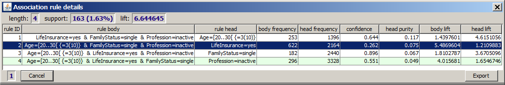
Clicking on a table row with the right mouse button opens a detail view of the association in a separate pop-up window. The detail view displays the n different possibilities to interpret the association as an association rule with exactly one item as the rule head. For each rule, the detail view contains the absolute support of the rule body and the rule head, the rule's confidence, the lift of the rule body pattern and the rule lift.
In the tool bar tab Result introspection the following options are available:
-
The information displayed at the left end of the tab contains the name of the data source and the number of patterns which are currently selected. When at least one pattern is selected, a mouse-click on the label Selected associations creates a pop-up window in which a SQL SELECT statement is displayed which corresponds to the currently selected patterns.
-
Next to this information there are two vertically positioned radio buttons with which you can switch between the default 'pattern view' and an an alternative 'rule view' in the result table displayed above. In the default display mode, each detected association pattern is represented by one single table row. In the alternative 'rule view', each pattern of n items is displayed in the form of n association rules, each one with another head item. Hence, the second variant is more complex but contains a lot of additional information for all the displayed rules. For displaying this information in the default pattern view, you would have to right-click on every single table row in order to display the row's detail view.
-
The next vertical pair of radio buttons determines what happens if several associations have been selectend and then the button
 is pressed. The button's purpose is to display those data groups which support the selected associations. The question is, does this mean the intersection or the superset of the supports of the single selected patterns? This question is answered by the choice made in these radio buttons.
-
The rightmost vertical pair of radio buttons has a similar function to the pair next to it: it specifies whether pressing the button dispays entire data sets or only the data record numbers or data group IDs of the data groups which support the selected patterns.
-
The button opens an additional window which shows the data groups on which the currently selected association patterns occur. Whether the new window contains full-width data records or only record or group IDs, and whether it contains the intersection or the superset of the data groups supporting the single selected patterns, is defined by the radio buttons described above.
-
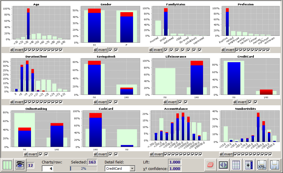
The button
 opens an additional window in which the data groups on which the currently selected patterns occur can be visually explored. Whether the new window contains the intersection or the superset of the data groups supporting the single selected patterns, is defined by the radio buttons described above.
The new window provides the entire functionality of the module multivariate analysis. The screenshot shown below explores the data groups which support the pattern of length 4 which has been taken as an example in the previously shown pictures. Then we have chosen the data field Creditcardas detail structure field. Now the blue and red bars are indicating how the non-credit-card-users and the credit card users behave within the customer group which support the selected pattern.
-
Using the button
 you can export the currently selected patterns, or all patterns if none has been selected, into a <TAB> separated flat text file, into a PMML
 AssociationModel or into a series of SQL SELECT statements.
-
Using the button
 you can export the data groups supporting the currently selected patterns into a <TAB> separated flat text file or into a spreadsheet in
 .xlsx format.
Pattern verification and significance assurance
At the end of the chapter on associations analysis we want to discuss how one can make sure that a detected pattern is a statistically significant pattern and not just a random statistical fluctuation, so called white noise, in the data. This issue is often completely left aside in traditional books on data mining and in many existing software packages.
Synop Analyzer provides two means for targeting this issue: one can calculate a so-called χ2 confidence level for each pattern, and one can perform one or more verification runs on artificially permuted versions of the original data which serve to define the so-called noise level and the associated 'Monte Carlo confidence' that the given pattern's statistical key measures exceed tht noise level, making it a significant pattern. In this section, the two confidence measures and their interpretation shall be discussed in detail.
As an example, let us look at one concrete association pattern which we have taken as an example several times in this chapter:
The highlighted sample pattern has length 4, absolute support (frequency) 163, relative support of 1.6%, a lift value of 6.64, the χ2 confidence of 1.000 and the Monte Carlo confidence of 0.58. What does that mean for the significance of the pattern, and why is the χ2 confidence of this pattern (and of most other patterns) much larger than the Monte Carlo confidence?
For answering these questions we start with remembering the definition of χ2 confidence. A pattern of n items with absolute support S has a χ2 confidence of x% if for each of the n items, the following holds: the appearance probability of the item in the presence of the n-1 other items of the pattern differs so strongly from the a-priori appearance probability of the item on the overall data that this difference is in x out of 100 cases greater than the difference in appearance probilities which results from comparing a randomly selected subset of S data groups to the entire data.
More familiarly spoken, that means roughly the following: x out of 100 association patterns which do not represent a statistically significant relation on the data and which have the same pattern length and support as the given pattern, would have a lift value closer to 1 than the given pattern. Inversely, this also means: even if a pattern has a χ2 confidence value of 0.9999, 1 out of 10000 randomly chosen noise patterns of the same length and support would have a lift value as strong as the given pattern.
A typical associations analysis - if not almost all items appearing in the detected patterns have been specified as 'required items' by the user - examines billions or even trillions of candidate patterns. Therefore, it is highly probable that e few random noise patterns make it into the displayed result which have a χ2 confidence of 0.999 or even 1.000.
In summary we can conclude: that a pattern has a χ2 confidence of 0.95 or higher is a necessary but not a sufficient condition for the pattern's statistical significance. The condition is only sufficient if the search space of candidate patterns during the analysis was very small, that means if only a few patterns were evaluated. In all other cases, one needs other significance measures for finally classifying a pattern as significant or not.
In these latter cases, the Monte Carlo confidence level, which is based on verification runs and permutation tests, gives a more reliable significance estimation. The method first calculates a 'maximum noise level' for each pair of (pattern length, support) based on all available verification runs. The maximum noise level takes into account all recorded lift, purity and core item purity values of the detected patterns on the verification data. From each triple (lift, purity, core item purity), a number NL(length,support) is calculated, and the maximum noise level MNL is the maximum of all recorded NL(length,support). For pairs (length,support) for which not enough patterns have been found within the verification runs, the maximum noise level is interpolated and estimated from neigbored MNL values.
Once the MNLs have been established, we calculate the corresponding quality number Q as a function of lift, purity and core item purity for each detected pattern on the real data and compare it to the MNL for the same length, support, lift, purity and core item purity. The Monte Carlo confidence is a function of Q minus MNL which is calibrated such that the result is 0.45 if Q equals MNL and 0.95 if Q equals 1.5 MNL.
Familiarly spoken, we can interpret the Monte Carlo confidence as follows: a value of about 0.5 means that on all verification runs not a single fluctuation pattern has been found with the same combined significance of the values pattern length, support, lift, purity and core item purity as the current pattern. This is a good evidence for the fact that the current pattern is statistically significant. The evidence becomes even stronger if the MC confidence goes towards 1.0. That means, our sample pattern, which has MC conf=0.58, is with high probability statistically significant, whereas the pattern below our example pattern in the result table could be random noise, even though its χ2 confidence is 1.000.
Applying association models to new data ('Scoring')
Association models can be applied to new data in order to create predictions on these data. For example, an associations model could use the click history of a web shop user to decide which product offers are to be shown to this user. Another associations model could serve as an early warning system in a production process, predicting upcoming problems and faulty products. A third associations model could classify credit demands into a high risk and a low risk group. This application of associations models to new data for predictive purposes is called 'scoring'.
In the current version of Synop Analyzer, associations models must satisfy a certain precondition for being usable for scoring: all association rules in the model must have rule heads ('then' sides) containing values of one single data field. This data field is called the target field of the model. In the three sample applications cited above (web shop, production monitoring, credit risk), the target fields could be ARTICLE, ERROR and RISK_CLASS.
If all rules of the model only contain information ('items') from one single data field, the precondition for scoring is trivially satisfied. If not, you can enforce the precondition by defining one or more required items of type Rule head when training the model. In this case, you must make sure all required head items are values or value ranges of one single data field.
You load and apply an associations model by first opening and reading the new data, by then pressing the button in order to start the associations analysis module and by then clicking the button Load model in the tab Scoring Settings of the tool bar at the lower end of the panel's GUI window.
In the following sections we will demonstrate the process of associations scoring with the help of a concrete example use case: using an associations model we want to predict the propensity of newly acquired bank customers to sign a life insurance contract.
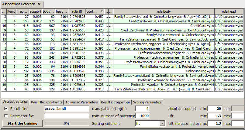
For this purpose, we load the sample data doc/sample_data/customers.txt. We keep the default data import settings with one exception: the number of bins for numeric fields (Bins:) is reduced from 10 to 5. Then we start the associations analysis module and train a model called assoc_li.mdl, using the following parameter settings:
-
Required item LifeInsurance=yes of type Rule head,
-
Incompatible items FamilyStatus=* and JointAccount=* (because these two fields are highly correlated),
-
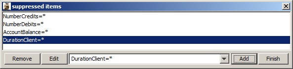
Suppressed items NumberCredits=*, NumberDebits=*, AccountBalance=* and DurationClient (because the information on accounting activity and acount balance are not reliably available for new customers and the duration of the business relationship is always 0)
-
Minimum absolute support 20, minimum lift 1.3, minimum lift increase factor 1.3.
The model trained with these settings contains 17 rules. The strongest rule predicts a probability of 45% that a customer with the properties given on the left side of the rule will sign a life insurance contract.
Now we want to use the generated model for predicting the propensity of 159 new customers for signing life insurance contracts. The new customers' data reside in the file newcustomers_159.txt. We load these data as a new Synop Analyzer data source. The value range discretizations of the numeric fields of the new data must be identical to the range discretizations that were in place when the model was created. In our case, we use the pop-up window Settings → Field discretizations to make sure the field Age has the range boundaries 20, 40, 60 and 80. For the field ClientID we specify the usage type group in the dialog Active fields.
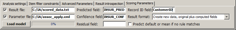
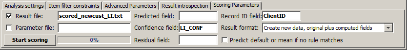
On this in-memory data source we start the associations analysis module and move to the tab Scoring Parameters in the tool bar at the lower end of the screen. Here, we enter the name of the file in which the scoring results are to be stored (scored_newcust_LI.txt), we define the scoring result data fields to be contained in that file and we specify that the new file should be a copy of the existing file newcustomers_159.txt plus the new computed data fields. (Create new data, original plus computed fields).
Since all association rules in our model predict the same value (LifeInsurance=yes), we do not need a new data field Predicted field. Instead, we are interested in the predicted probability of that value, therefore we define a Confidence field and call it LI_CONF. For being able to identify the single customers in the new data, we make sure the key field ClientID is contained in the new data and serves as Record ID field.
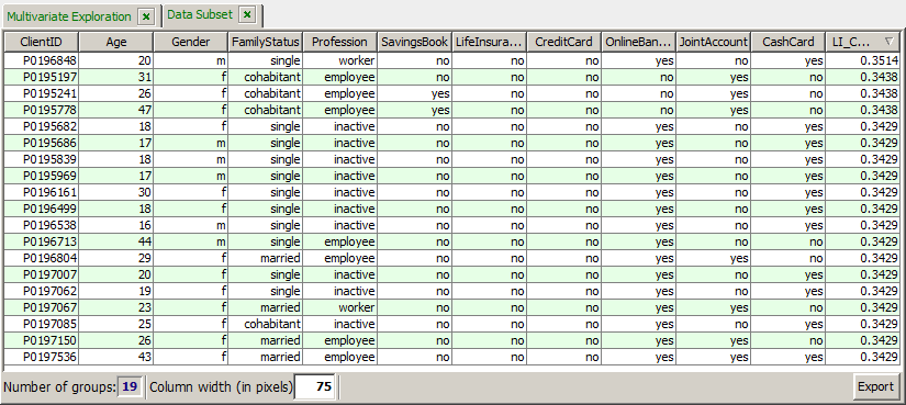
By means of the button Start scoring we create the scoring results, write the desired result file to disk and open the resulting data as a new in-memory data source in Synop Analyzer, that means as a new tab in the left column of the Synop Analyzer workbench.
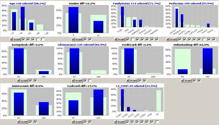
We introspect the scoring result data with the module 'multivariate exploration'. We see that the model has created a non-empty propensity probability for 39 of the 159 new customers. But some of these 39 customers should be filtered out because they already have a life insurance, they have an age of 60 or more years or because they are children or retired persons. There remain 19 new customers which are interesting for selling life insurance contracts:
Via the button we submit the selected 19 data records to a last visual examination. Then we can use the button Export to save the resulting list to a flat file or Excel spreadsheet, or we can use the main menu button Report to create a HTML or PDF report.