Tutorial: Customer Intelligence

Content

Business Case
Advantages of the Synop Analyzer approach to Customer Intelligence
Sample Data used in this Tutorial
Step 1: Loading the Data
Step 2: Obtaining a First Overview
Step 3: Multivariate Interactive Data Exploration
Step 4: Customer Intelligence with Multivariate Data Exploration
Step 5: Campaign Plannung and Target Group Selection
Step 6: Detailed Look at the Interrelation of two Fields
Summary

Business Case

Understanding the customers and their needs is essential for every enterprise in today's economic environment, which is largely characterized by supply surpluses and selective and critical customers who are well aware of the fact that they can choose among many different products and vendors.

With its intuitive and highly scalable multidimensional data exploration capabilities, Synop Analyzer provides a powerful tool for a data-driven approach to understanding customer behavior, and for deriving sales and marketing strategies from these insights. In this tutorial, we demonstrate this unique approach using bank customer master data with a view to analyzing those customers with large amounts of money on their current accounts. The questions to be answered are as follows:

• Can customers with a high average balance on their current account be clustered into several homogeneous groups of people with similar demographic or buying attributes? Which attributes describe these clusters?
• Can we derive sales and marketing strategies, up-selling actions or other sales or marketing campaigns from these findings?

Other application scenarios for this type of interactive data exploration comprise:

• Marketing campaign planning: select suitable target groups and the best matching contact channel for each group within a marketing campaign for a specific product or service offering.
• Sales planning and marketing strategies.
• Sales controlling and success tracking: which sales unit or sales representative performed better/worse than their peer groups and why? In what respect did the successful sales units differ from the less successful sales units?
• Sales force education, training and support: provide each sales representative with individual hints and success strategies tailored towards the specific characteristics of the sales representative's client group, region, product portfolio, time of the year etc.

Advantages of the Synop Analyzer approach to Customer Intelligence

Compared to other methods and tools for customer data analytics, Synop Analyzer offers the following advantages:

• Ease of use: Unlike many other interactive 'drill-down' tools, Synop Analyzer does not require elaborate data preprocessing or data modeling (e.g. the setup of a cube model and a cubing engine) prior to starting the exploration itself. Just connect to a raw data table or view, or load an Excel sheet or flat file and start the exploration.
• Speed: Typically, you will have your exploration results only minutes after connecting to a table or file. This quick 'time to result' approach can be achieved because Synop Analyzer automatically performs the necessary data attribute selections and data preparations (e.g. value discretizations into suitable ranges or intervals), and because the single drill-down and data selection steps are truly 'interactive' in the sense that they return their results within fractions of a second, even on the largest customer data set.
• Unique combination of interactive data exploration and data mining: together with the interactive data exploration capabilities demonstrated in this tutorial, Synop Analyzer offers a set of powerful data mining features whose capabilities complement the features demonstrated in this tutorial. Separate tutorials are available for these features.
• Performance: due to its data compression scheme, its in-memory data handling and its powerful analytics algorithms, Synop Analyzer is able to explore data tables of 10 million customers or more on a simple PC or notebook with 'real-time' response times of less than a second.
• Scalability: Synop Analyzer's analytic engine supports multithreading, multi-core CPUs and multi-CPU servers with almost perfectly linear speedup. That means, if you double the number of concurrent users, doubling the number of available CPU cores and the available RAM on your analytics server keeps the engine's response times unchanged.
• Seamless integration into the existing IT and business analytics infrastructure: Synop Analyzer interacts with databases, reporting systems and other enterprise applications via standard interfaces such as JDBC, web services (SOA), or XML. You can define and deploy Synop Analyzer standard processes in the form of automatically running batch jobs, database stored procedures or system services.
• Competitive TCO (total cost of ownership) due to little demand for hardware, software and administrative resources and flexible pricing. This makes Synop Analyzer suitable for virtually all companies, regardless of IT department sizes and budgets.

Sample Data used in this Tutorial

In this tutorial, we analyze a master data file containing customer data of 10,000 bank customers. The data records are available in the form of the <TAB> separated flat file doc/sample_data/customers.txt which contains 15 attributes such as the customers' age, profession, family status, customer history, assets and the banking services they are using.

Step 1: Loading the Data

In this section, we use the Synop Analyzer module Input Data to load a flat text file into Synop Analyzer. We start the Synop Analyzer workbench (double-click on the executable batch file SynopAnalyzer) The main panel of the Synop Analyzer graphical workbench opens up, showing a bipartite empty canvas. The left column will later display some basic properties of all data sources which have been opened in Synop Analyzer. In the right part of the canvas you can run various data analysis modules.

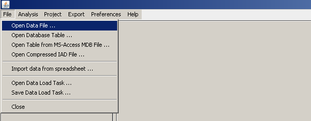
Using the main menu item File we can select a flat text file to be opened:

Clicking on File → Open Data File opens up a file chooser dialog in which we select the input data file doc/sample_data/customers.txt.

Now the left part of the screen displays some basic properties of the data. In the following, we will call that part of the screen the input data panel. At the beginning of each data exploration with Synop Analyzer, the data has to be loaded into a binary compressed representation which resides in the computer's RAM. This loading process is started by pressing the Start button in the input data panel. In addition, the panel provides a couple of input fields and buttons for manually adjusting the data import process. For now, we want to load the input data using default import settings, therefore we directly press the Start button.

Note: every data specification and analysis module of Synop Analyzer has a context-sensitive help system in the form of a 'mouse-over' function which opens up explaining texts for a button, input field or output element whenever you place the mouse pointer on a label, field or button.

Note: you find more explanations on the advanced parameters for the data loading in the module description of the Input Data Panel, for example how to modify the number of value ranges or the range boundaries shown in the histograms for the numeric data fields.

Note: by opening the pop-up dialog Show advanced options in the input data panel and by activating the checkbox Create persistent data file you can create a permanent version of the compressed data on disk. The compressed file has only about 8% to 10% of the initial data file size. This data file can be re-read in later analysis sessions, which for large files is much faster than reading and compressing the corresponding flat file each time.

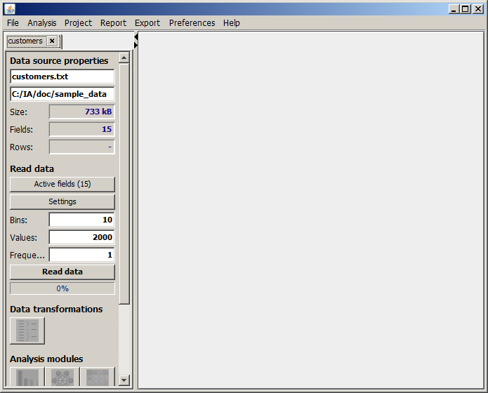
While the blue progress bar proceeds from 0 to 100%, the data is read, compressed and stored in memory. On large data sets, on a typical PC with one CPU, about 1 GB of data can be read and compressed per minute.

When the data reading is finished, the buttons in the lower part of the input data panel change their appearance, indicating that the data are now ready to be used. But In our case we first get a warning message:

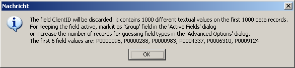
The message tells us that the column ClientID is a key-like field which contains a unique value in each data row. Those fields are not suitable for creating value distribution statistics or for using them as selection criterion within interactive data analysis steps. Therefore, the data field is being deactivated by default.

Even though we agree that we don't want to see ClientIDs in statistics or multivariate data explorations, we would like to maintain the field in the imported data because the values serve as unambiguous identifiers (keys) for the data sets: Whenever we have selected an interesting set of data records, we need their ClientID's in order to unambiguously identify the selection's data records.

Therefore we follow the advice of the warning message and open the pop-up dialog Select active fields. In the leftmost column (Active), we re-activate the field ClientID. In the column Usage we define the field to be the group field:

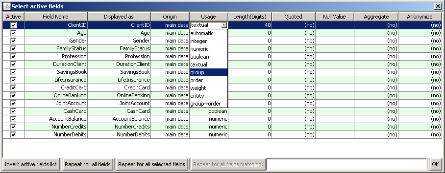
Now we close the pop-up window with the OK button and reload the data by pressing Start. This time, the data reading succeeds without warning messages. Once the data are available in memory, the buttons in the lower part of the input data panel on the left side of the screen become usable. We first press the button Statistics and Distributions in order to get a quick overview of the available data fields and the data quality.

Step 2: Obtaining a First Overview

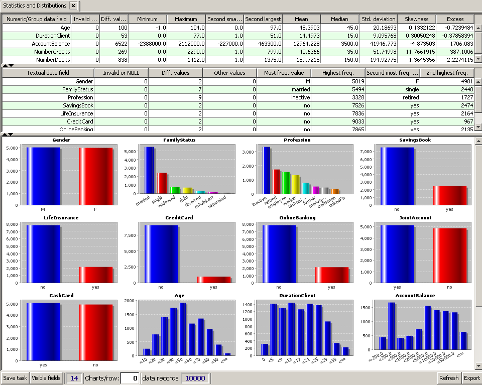
The main purpose of the 'Statistics and Distributions' panel is to gain a first overview on the kind of information contained in the data. Furthermore, obvious data quality issues become visible, such as fields with many missing or invalid values, fields with erroneous values (e.g. negative age, profession="xxx", etc.). A more sophisticated data quality checking can be performed using the module Deviations and Inconsistencies which is described in a separate tutorial.

The panel 'Statistics and Distributions' consists of three parts separated by horizontal bars. By mouse-drawing these bars, or by clicking on the arrow symbols on the left end of the bars, you can change their size and minimize or maximize each of the three parts.

The first part shows an overview statistics on the active numeric data fields: the original and the displayed field name, the number of rows with missing or invalid (non-numeric) content, the number of different values, and the basic statistical distribution measures such as mean, median, minimum, maximum, standard deviation, etc.

The second part shows an overview statistics on the active textual and Boolean fields: the field name, the number of rows with missing content, the number of different values, the most frequent value with its frequency and the second most frequent value with its frequency.

The third part displays a graphical representation of each field's value distribution in the form of one histogram chart per data field.

For the numeric fields, Synop Analyzer has automatically chosen suitable discretizations into the number of bins that has been specified in the field #bins (numeric field) on the input data panel. Depending on a field's actual value distribution statistics, Synop Analyzer either chooses a binning into equidistant intervals, or a logarithmic binning. In the data used here, the field Age, which has a value distribution close to a Gaussian 'normal' curve, has been discretized into equidistant intervals. The field AccountBalance, on the other hand, has been discretized logarithmically. The software has automatically detected that this field's value distribution is not suitable for equidistant binning because it has its center between -200 and 1000 but also a significant 'fat tail' at much higher values of more than 10000 or even 50000.

Note: you find more explanations on the module Statistics and Distributions in the module's documentation.

For now, we are satisfied with what we see: the 14 non-group fields apparently contain reasonable values and value distributions, and there are no missing or invalid values. Also, the default binnings and value range definitions performed by Synop Analyzer are suitable for the planned analysis steps. Therefore, we do not further fine-tune the data loading options and directly start a multivariate data exploration.

Step 3: Multivariate Interactive Data Exploration

Pressing the button Multivariate Exploration opens a new panel, consisting of one histogram chart per active data field and a tool bar at the lower edge of the tab. Each histogram chart compares a field's value distribution on the currently selected subset (blue bars) to the field's value distribution on the entire data (light green bars).

By clicking on one of the checkboxes below each chart, you can define a value selection for the corresponding data field. For example, in order to select only those customers who are married, click on the leftmost checkmark below the chart for the field MaritalStatus (this selects all but the married customers), the click on the invert button (this inverts the previous selection, and hence selects only the married customers):

The tool bar at the bottom of the screen shows some overall statistics of the current selection:

• The progress bar on the left and the adjacent text field Selected show the size of the currently selected subset of the data: once as a percentage of the entire data, once the absolute number of selected data record.
• The text field Lift indicates whether the combination of field value ranges defining the current selection 'attracts' or 'repulses' each other. lift values larger than 1.0 (less than 1.0) indicate that the different selected value ranges occur more (less) frequently together than expected in the case of statistical independence.
• The text field χ²-Confidence contains the statistical confidence that the selected subset differs significantly from the entire data in at least one data field's value distribution. (More formally spoken the value is the confidence level with which the hypothesis 'The currently selected subset has the same value distribution in all data fields as the entire data' is rejected by a χ² significance test.)
• The input field Charts/row defines how many histogram charts are displayed in one screen row.
• The Export button opens a 'save file' dialog which stores a snapshot of the current state of the analysis to a spreadsheet in .xlsx file format (MS Excel^© 2007+ format).

The fields' histogram charts can have two different appearances, depending on whether or not a value range selection has been performed for the field:

• Fields for which certain values have been selected, others deselected, have a blue title which shows the field name and the number of data records which are covered by the field's current value selection. In the figure above, 5494 records with MaritalStatus=married have been selected. Therefore the histogram for the field has a blue title text.
• Fields for which the value range has not been restricted are shown with black title. The title then contains the field name and a percentage number which indicates how much the blue and the light green bars differ, or in other words: how much the field's value distribution on the selected subset differs from the field's value distribution on the entire data. From the figure shown above we learn that married and unmarried customers differ most strongly on the field JointAccount (33.9%) and most weakly on the field LifeInsurance (0.2%).

The y-scale of each histogram contains a percentage number indicating the relative frequency of the single values or value ranges. For example, looking at the histogram for Profession in the picture above we see that on the overall data, about 33% of all data records have Profession=inactive, whereas on the currently selected subset (MaritalStatus=married) only about 21% of the selected data records have the value Profession=inactive.

Step 4: Customer Intelligence with Multivariate Data Exploration

Let us now assume that the multivariate exploration has been started with the goal to analyzing those customers who have large sums of money on their giro bank account. The question is:

• Do these customers have typical attributes? Can they be grouped into some homogenous clusters?
• Which other banking services are they using?
• Are there up-selling potentials for promoting other banking services to those customers?

In order to answer this question, we first undo our current selection by pressing the 'all' button for the field MaritalStatus or the Clear button in the tool bar.

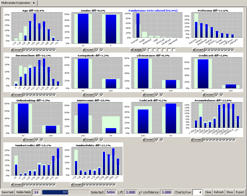
Then we select only those customers with an AccountBalance above 20000: click on the two rightmost checkboxes below the histogram for AccountBalance, then click on the invert button.

How did this selection of the 1950 customers with the highest average balance score influence the other fields' value distributions? To answer this we re-arrange the histograms by decreasing difference between the selected and the overall data: we click on the Visible fields button and then on Sort by → relative difference (see the picture below).

We see that the most significant changes are:

• A shift in the Age distribution towards higher ages (not very surprising)
• A significant over-representation of the professions Profession=pensioner (also not very surprising) and Profession=farmer.

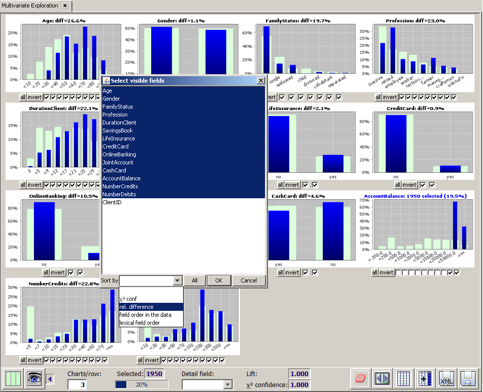
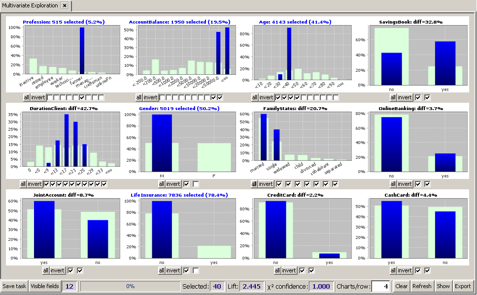
This last observation seems the most interesting to us. We want to focus on those farmers with an account balance of more than 20000 Euros. We therefore narrow down the existing selection by clicking on the fourth checkmark from the right below the histogram for Profession, then on the invert button. This selects only the value Profession=farmer.

Then we again open the Visible fields dialog, sort the fields by 'relative difference' and hide the two fields NumberCredits and NumberDebits, which are of little interest in the analysis we are performing. (Keep the <CTRL> key pressed while clicking on the two field names in order to remove them from the list of visible fields.)

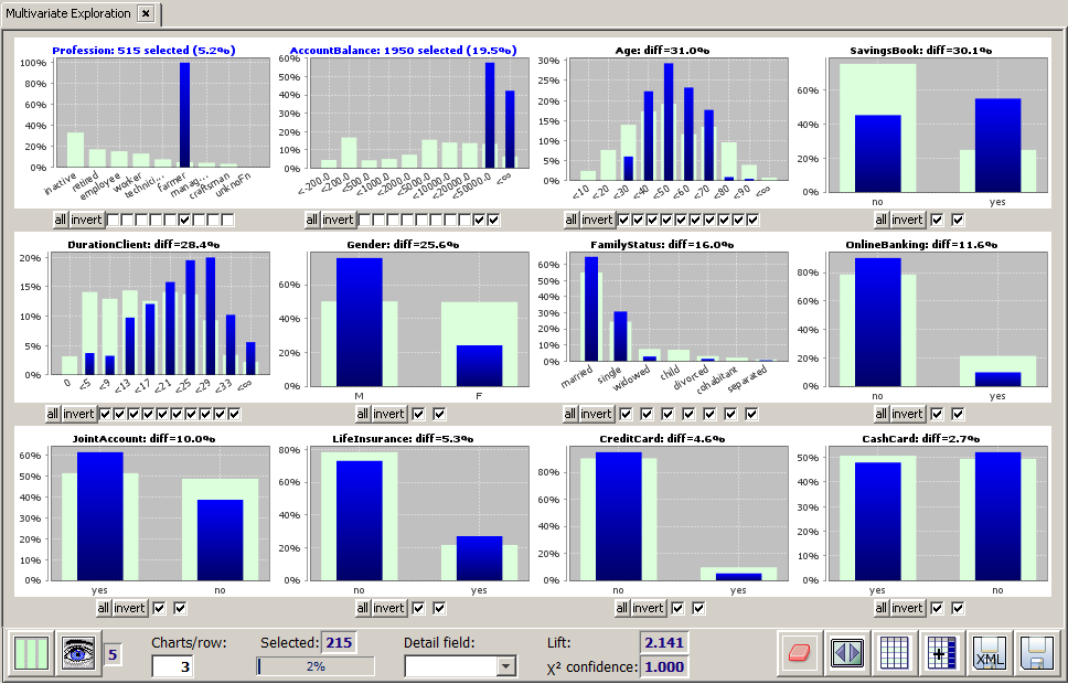
Interestingly, this refinement of the previous selection pushes the age distribution back to the younger age groups (see picture below). Hence, among all customers with high amounts of money on their giro bank account, the farmers rank among the youngest. Furthermore, we see that Gender=m and MaritalStatus=married and MaritalStatus=single are strongly over-represented in this group. And, what is also interesting, most of those 'rich' farmers do not have a life insurance, at least not from our bank. On the other hand, they seem conservative (many of them have a SavingsBook, few of them use OnlineBanking), and they are very loyal customers (DurationClient strongly above average).

Step 5: Campaign Plannung and Target Group Selection

We believe that in the previous section we have identified a very promising target group for an up-selling campaign. Our idea is that we want to further narrow down our selection to the married male farmers below 40 years who do not yet have a life insurance from our bank. This group seems to be an excellent target group for a phone call or a personal visit with the goal of speaking about a life insurance for protecting the family:

• The group seems to be prosperous.
• The group is relatively young.
• The group is married and probably has children.
• The group has a dangerous profession which demands financial protection of wife and descendants in case of an illness or accident.
• The group has an above-average propensity to have a life insurance.

We perform the selection as described above by clicking on the suitable checkboxes and buttons below the histograms for MaritalStatus (married), Age (<40), Gender (m), LifeInsurance (no).

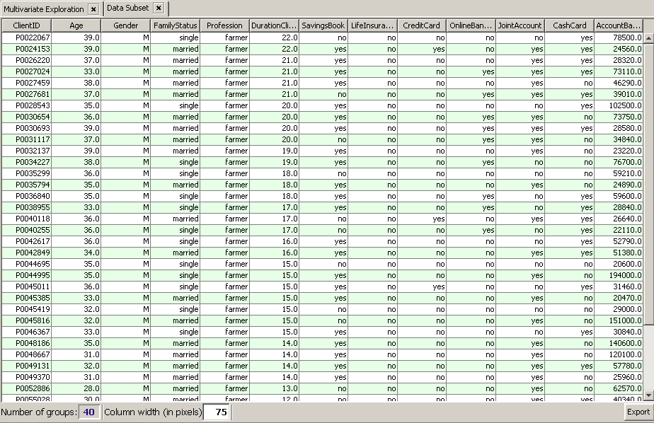
We notice that the remaining group consists of 40 customers, a reasonably small number of customers for being contacted by one sales representative. As a final check before starting the campaign, we would like to introspect the 40 selected data records. To this purpose, we click on the Show button on the right end of the tool bar. This brings up a new panel showing the selected data records:

We are satisfied with the selected target group for the sales campaign. Now we want to start the campaign by sending both the analysis rationale and the selected target group to the colleagues who will be responsible for running the campaign but who do not neccessarily have access to Synop Analyzer. We press the Export button on the right end of the tool bar of the multivariate analysis panel. A 'Save file' dialog opens up in which we can specify the name of the spreadsheet file into which the analysis results (in the form of png graphics objects) and the selected customer data records will be written.

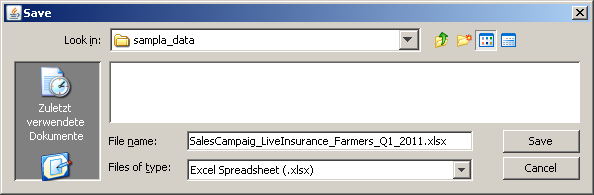
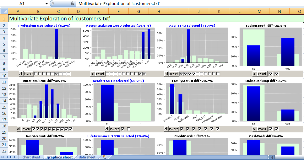
That file can later be opened in MS Excel^© or another front-end by the sales representative who will be in charge of contacting the selected people. It contains two tabs with the analysis summary and one tab with the selected data sets:

Step 6: Detailed Look at the Interrelation of two Fields

Our successful identification of a subgroup of farmers with a particularly high average balance on their giro accounts motivates us to study the interrelation between a customer's profession and its average balance it more detail.

In the input data panel on the left side of the screen we click on the Bivariate Exploration button. A new Bivariate Exploration panel opens up. The new tab is vertically split into two columns. In the left column, you can select the two data fields whose interrelation you want to study. In the right column, you see the resulting bivariate statistics for your selection. Per default, the first two active fields in the data are interrelated. We want to see the fields Profession and AccountBalance instead. Therefore, we use the two selection fields under 'x-axis' and 'y-axis' and select the fields Profession and AccountBalance.

By default, each field is divided into two ranges (classes) for the bivariate analysis. For the field PROFESSION that is not what we want to have. Instead, we want to treat each sufficiently frequent profession value as a separate class. Therefore, activate all checkboxes except the rightmost one below the histogram for field Profession. This treats the 7 most frequent profession values as separate classes and creates one summary class for the remaining values craftsmen,... and unknown (see picture below).

The second field we are interested in is the AccountBalance field. Here, we activate all but the third and fourth checkbox below the histogram. This creates the value ranges <-200, -200...200, 200...2000, 2000...5000, 5000...10000, 10000...20000, 20000...50000 and ≥50000. (see picture below).

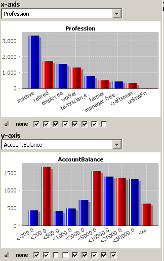
The right-hand side of the panel now shows two bivariate value frequency plots of AccountBalance as a function of Profession.

The upper chart shows which combinations of AccountBalance and Profession appear more (green) or less (red) frequently than expected if the two fields were statistically independent.

Some of the findings are not very surprising: professionally inactive customers have often an account balance near 0, pensioners and managers often have very high account balances, etc. But there are also some surprising findings, for example that managers are strongly over-represented among the customers who have a significantly negative account balance... Einige der Ergebnisse überraschen nicht wirklich: beruflich inaktive Kunden haben oft einen Kontostand in der Nähe von 0, Rentner und Manager öfter sehr hohe Kontostände etc. Aber es gibt auch Überraschungen, z.B. dass Manager stark überrepräsentiert sind in der Gruppe der Kunden mit signifikant hohem negativen Kontostand...

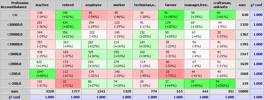
The black 'sum' row and column respectively contains the total number of data records which have the field value given in the column or row header. The black number in the right corner is the total number of records (or, if the check box 'ignore invalid/missing values' in the left part of the panel has been selected, the total number of records which have a valid value in both considered fields.

The meaning of the χ²-conf columns and rows as well as some other more advanced features of the bivariate exploration modules are explained in a separate section of the documentation.

The lower part of the right column contains a bivariate plot of absolute value pair counts, the area of each blue circle being proportional to the represented number of records which have the field values at the position (x,y):

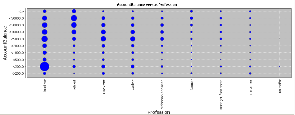
This kind of plot helps in identifying quickly the 'hot spots' of the value pair distribution, i.e. the most frequent field value combinations.

Summary

In Summary, we have demonstrated how customer data can be intuitively explored using Synop Analyzer. The exploration required neither an elaborate data preprocessing nor sophisticated statistical or tool handling skills and created insights and evidence which can be immediately applied for marketing campaign planning, sales controlling and other management tasks.